Graph Neural Network- GNN#
A powerfull tool for Capturing Dependencies in Graph Structured Data.
The motivation behind using graph convolutions#
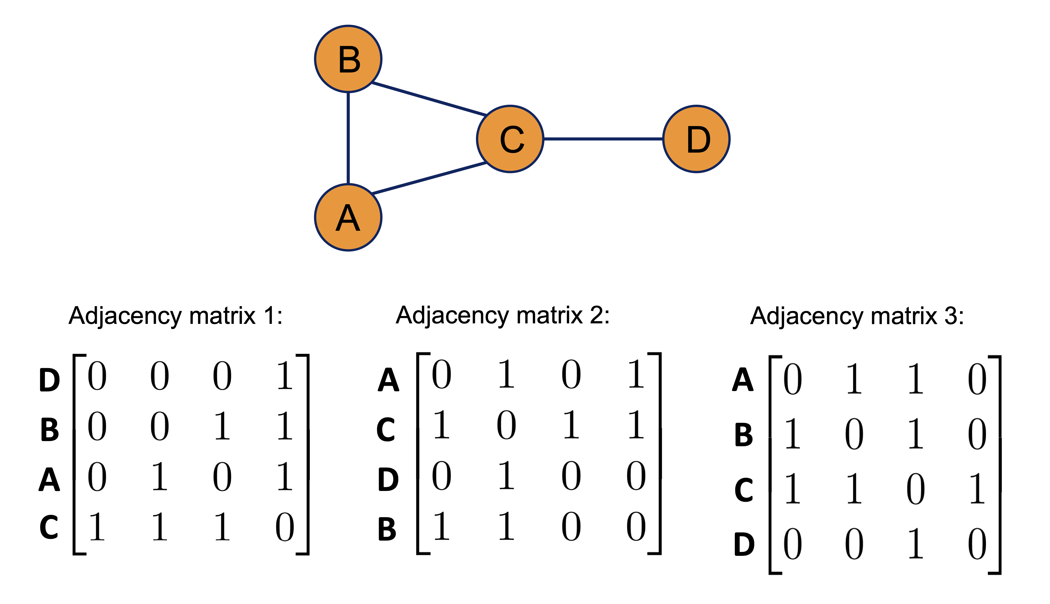
Graphs are invariant under node ordering. Therefore, as shown below, all of the adjacency matrices represent the same graph.
from IPython.display import Image, display

Image(filename='images/GNN_graph.png', width=500)
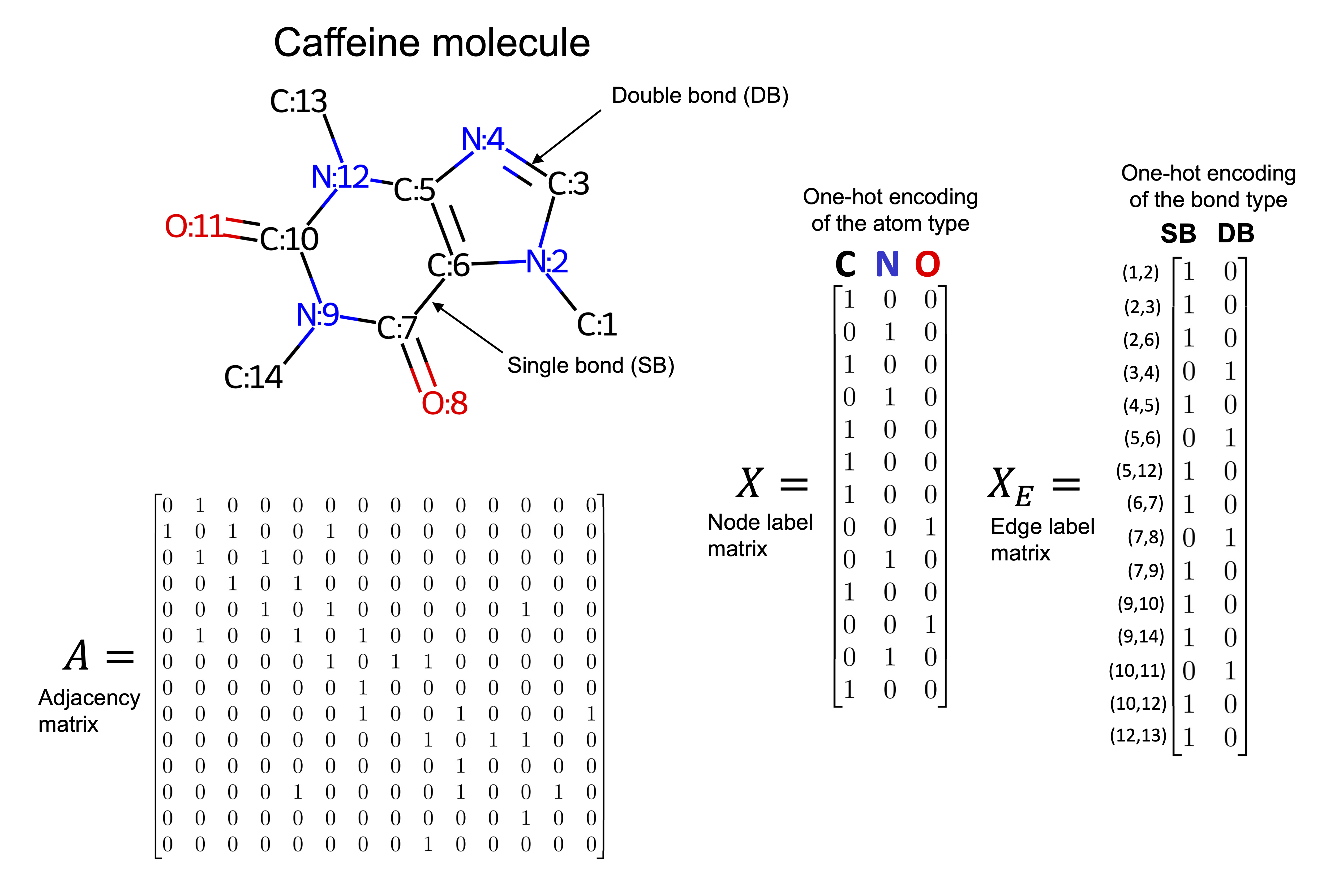
An Example: Representing molecules as graphs#
Molecular structures in two or three dimensions can be naturally represented as graphs. For instance, the caffeine molecule shown below can be modeled by treating each atom as a node in the graph. Edges between nodes represent chemical bonds, such as single or double bonds.
Each node is associated with a three-dimensional feature vector describing the properties of the corresponding atom, while each edge has a two-dimensional feature vector that captures the characteristics of the bond. In this example, node features encode the atom type, and edge features encode the bond type. Depending on the specific task and the available chemical information, the definitions of node and edge feature sets can be adapted accordingly.
Image(filename='images/GNN_Molec.png', width=500)
Understanding graph convolutions: Implementing a basic graph convolution#
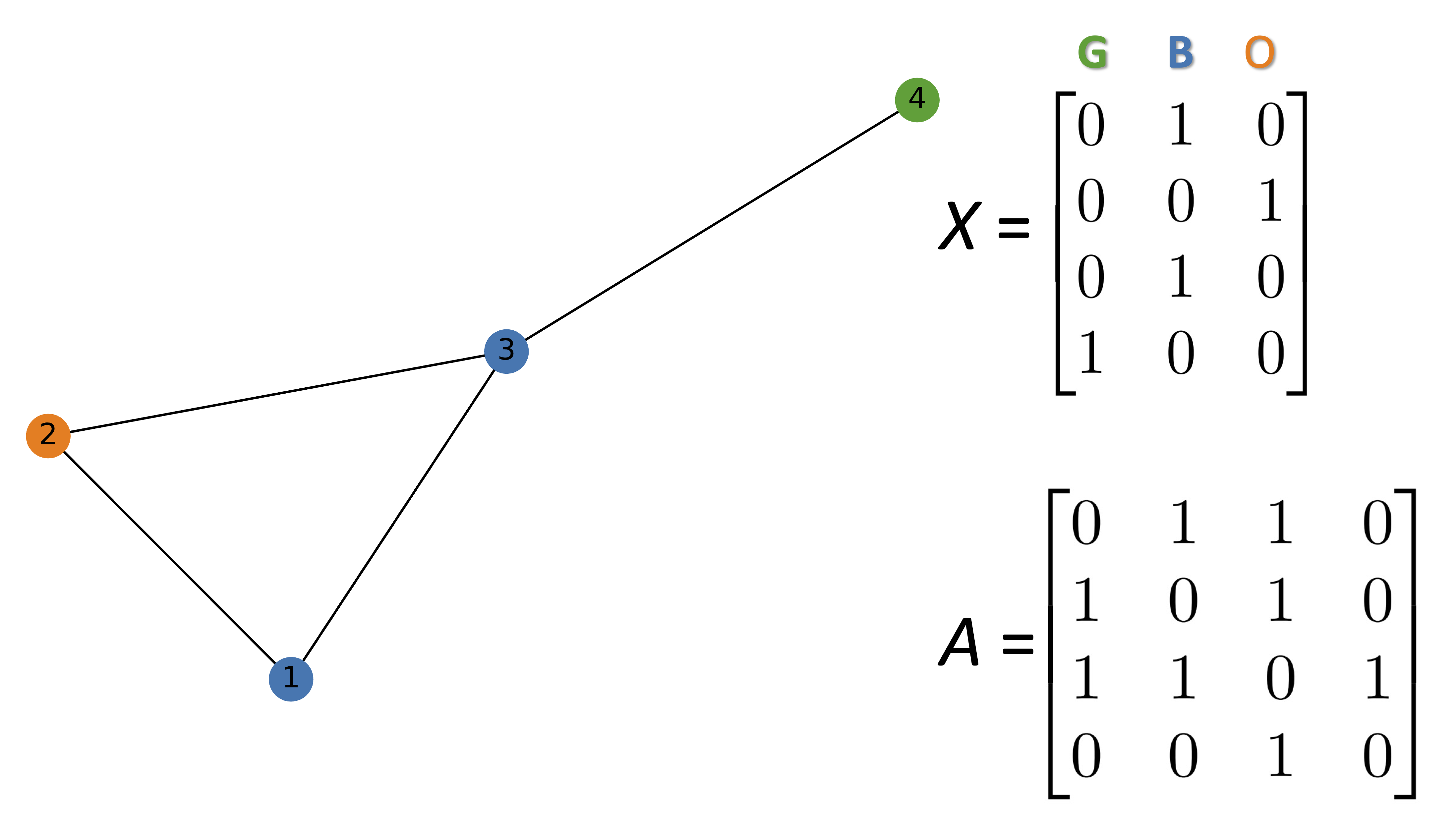
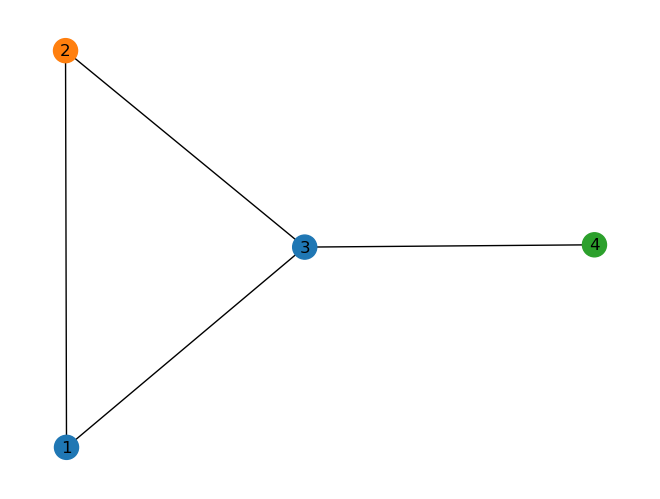
In the followig simple example, each node has a three dimensional representaion. Each row represents the features of that specific node.
Image(filename='images/GNN_graph2.png', width=500)
The follwoing code generate the above graph using networkx library.
import networkx as nx
import numpy as np
import scipy
G = nx.Graph()

#Hex codes for colors if we draw graph
blue, orange, green = "#1f77b4", "#ff7f0e","#2ca02c"

G.add_nodes_from([(1, {"color": blue}),
                  (2, {"color": orange}),
                  (3, {"color": blue}),
                  (4, {"color": green})])

G.add_edges_from([(1, 2),(2, 3),(1, 3),(3, 4)])
A = np.asarray(nx.adjacency_matrix(G).todense())
print(A)
[[0 1 1 0]
 [1 0 1 0]
 [1 1 0 1]
 [0 0 1 0]]
def build_graph_color_label_representation(G,mapping_dict):
    one_hot_idxs = np.array([mapping_dict[v] for v in
                             nx.get_node_attributes(G, 'color').values()])
    one_hot_encoding = np.zeros((one_hot_idxs.size,len(mapping_dict)))
    one_hot_encoding[np.arange(one_hot_idxs.size),one_hot_idxs] = 1
    return one_hot_encoding

X = build_graph_color_label_representation(G, {green: 0, blue: 1, orange: 2})
print(X)
X.shape[1]
[[0. 1. 0.]
 [0. 0. 1.]
 [0. 1. 0.]
 [1. 0. 0.]]
3
color_map = nx.get_node_attributes(G, 'color').values()
nx.draw(G, with_labels=True, node_color=color_map)
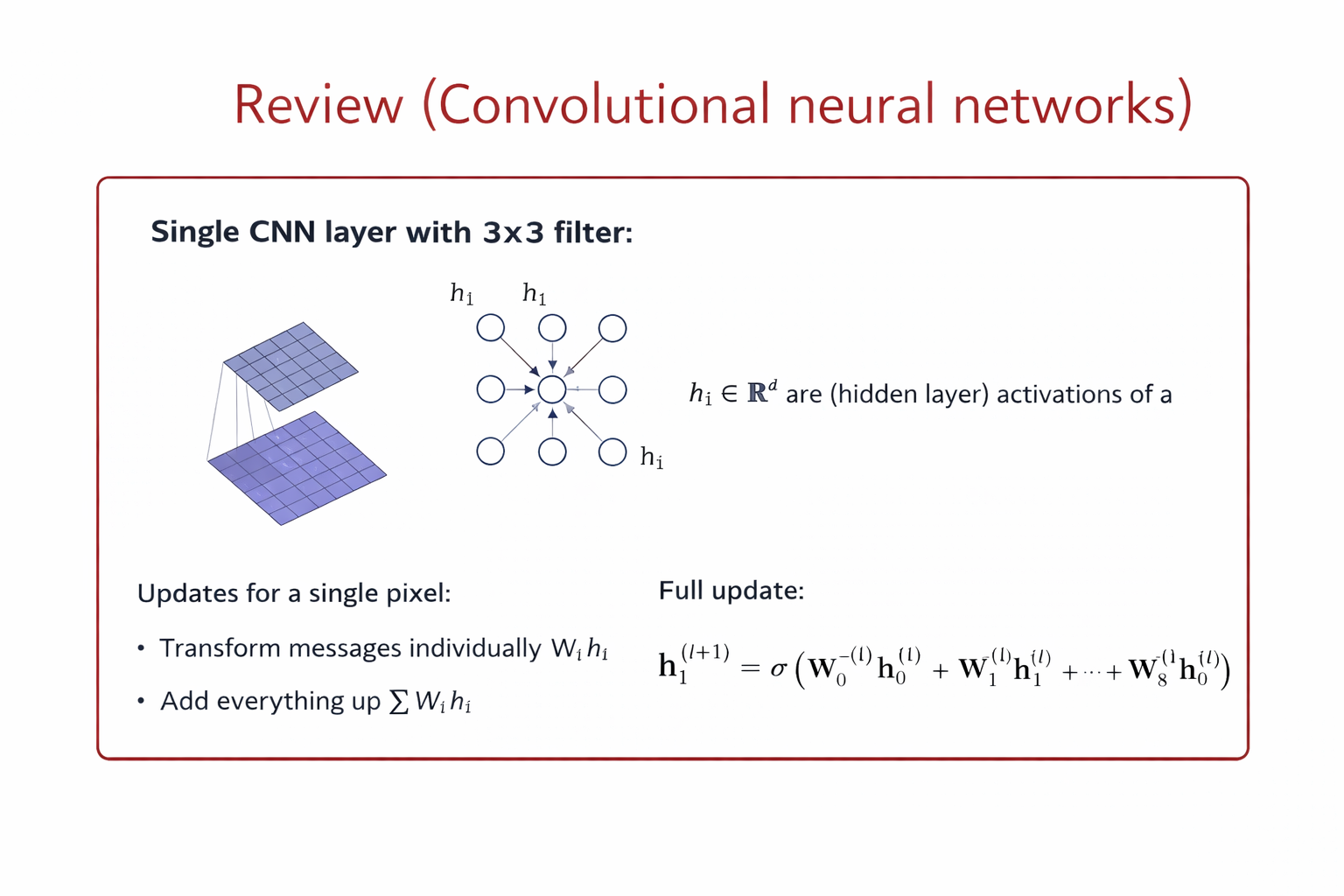
Convolution in CNNs (Grid-Structured Data) Let \(x_{i,j} \in \mathbb{R}^F\) denote the feature vector at pixel location \((i,j)\). A convolutional layer with a \(k \times k\) kernel computes:
\( h_{i,j}^{(l+1)} = \sigma \left( \sum_{(u,v) \in \mathcal{N}(i,j)} W_{u-i, v-j}^{(l)} , x_{u,v}^{(l)} + b^{(l)} \right) \)
Key properties
Neighborhood: fixed spatial window (e.g., 3×3)
Parameters: shared kernel weights
Ordering: fixed by grid structure
Operation: local weighted sum
Convolution in GNNs (Graph-Structured Data) Let \(h_i \in \mathbb{R}^F\) be the feature vector of node (i), and \(\mathcal{N}(i)\) its neighbors.
A generic graph convolution layer is:
\( h_i^{(l+1)} = \sigma \left( W_{\text{self}}^{(l)} h_i^{(l)} + \sum_{j \in \mathcal{N}(i)} W_{\text{nbr}}^{(l)} h_j^{(l)} \right) \)
or more generally:
\( h_i^{(l+1)} = \sigma \left( \text{AGGREGATE}_{j \in \mathcal{N}(i) \cup {i}} \big( W^{(l)} h_j^{(l)} \big) \right) \)
Key properties
Neighborhood: defined by graph edges
Parameters: shared across all nodes
Ordering: permutation-invariant
Operation: message passing + aggregation
Mathematical Correspondence#
CNN |
GNN |
|---|---|
Pixel |
Node |
Spatial neighbors |
Graph neighbors |
Sliding window |
Message passing |
Kernel weights |
Shared transformations |
Translation invariance |
Permutation invariance |
Why This Is a Convolution#
Both CNN and GNN layers:
Aggregate local neighborhood information
Use shared parameters
Build hierarchical representations by stacking layers
A graph convolution generalizes classical convolution from regular grids to arbitrary graph structures, replacing spatial locality with topological locality.
Image(filename='images/GNN_intro.png', width=800)
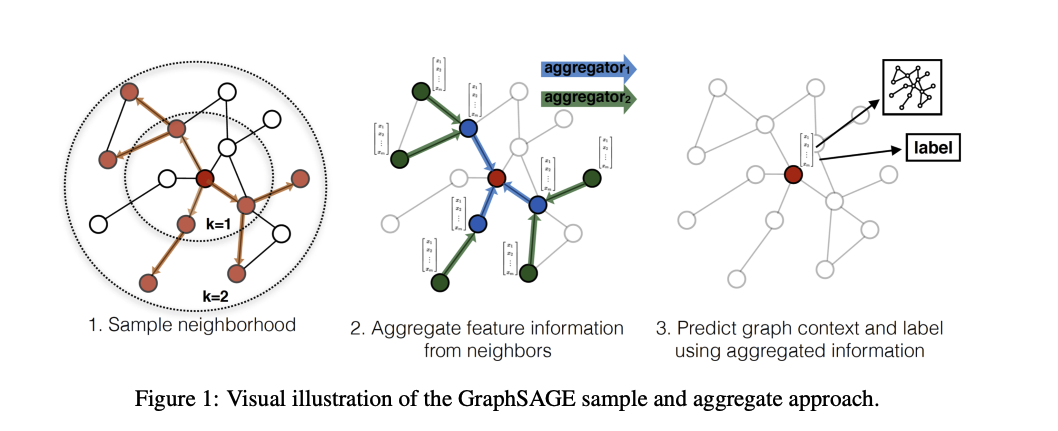
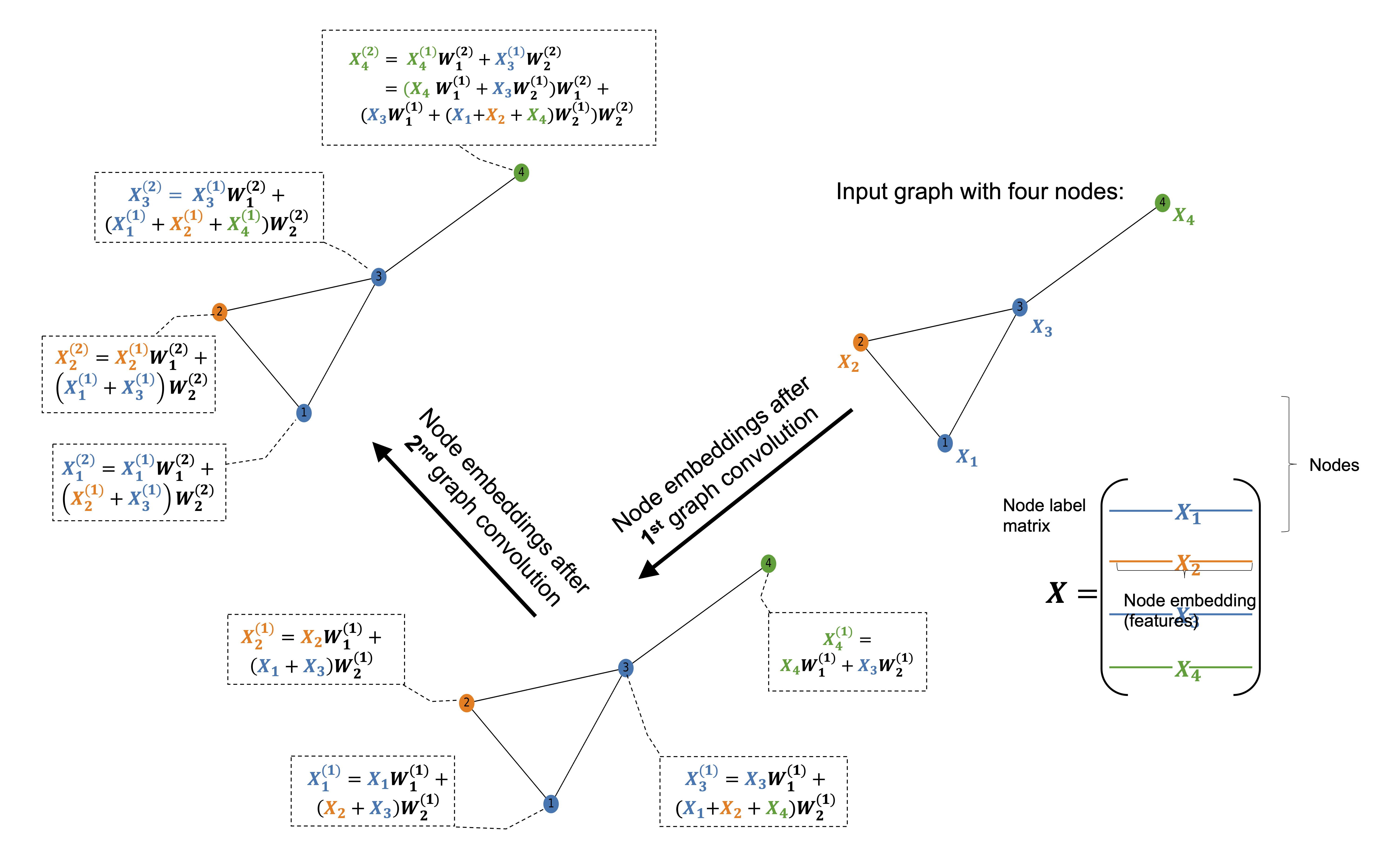
The figure illustrates how the first graph convolution layer aggregates information from immediate neighbors, while the second layer captures information from neighbors of neighbors.
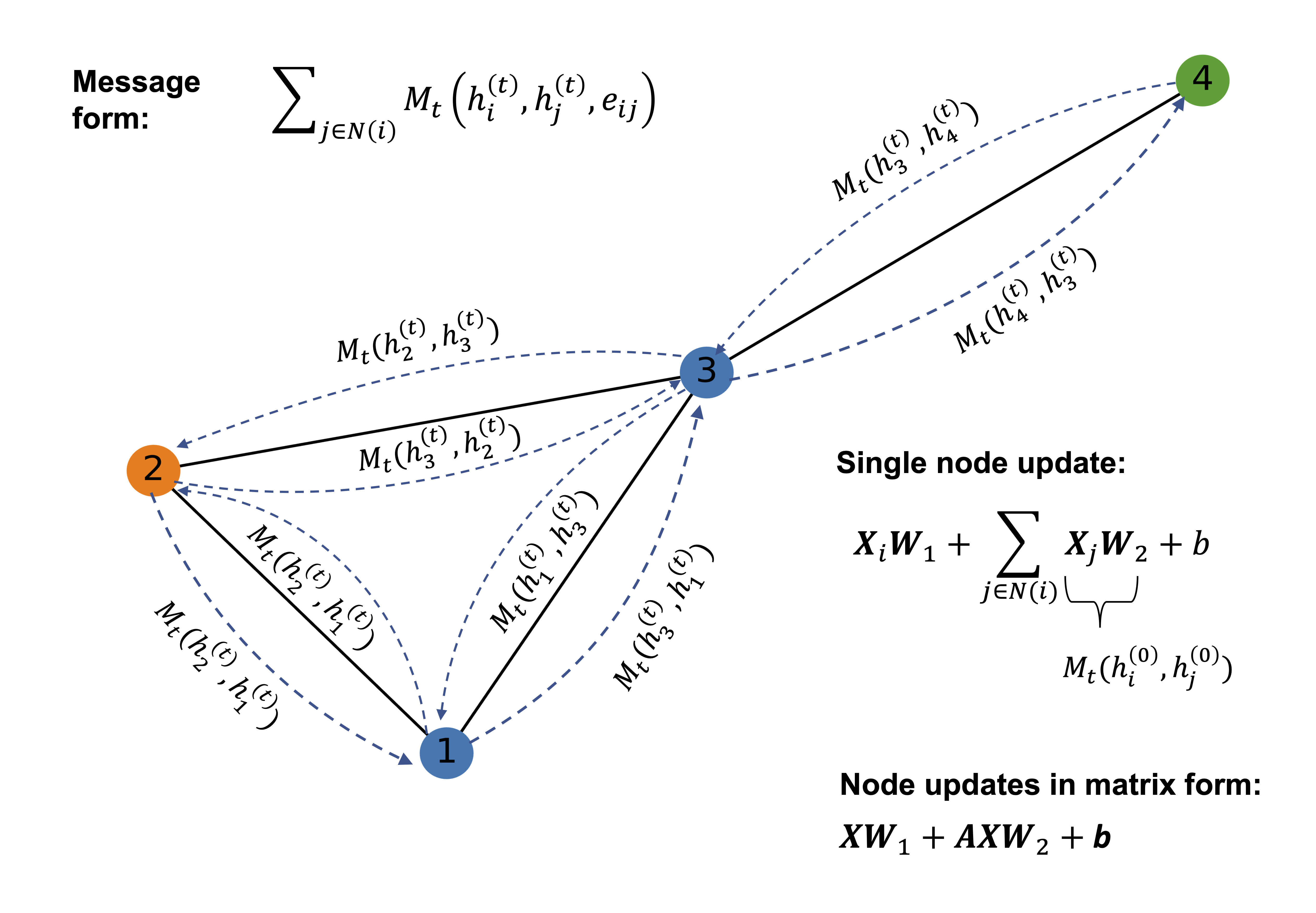
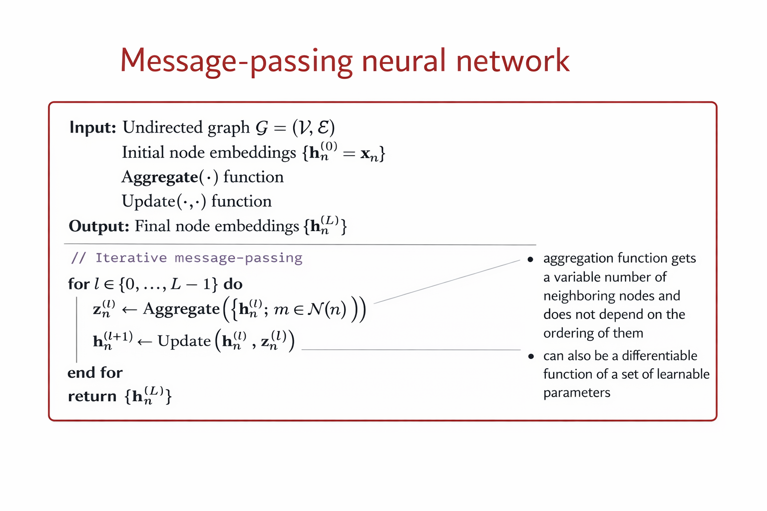
In a graph convolution, each node updates its representation by collecting and combining feature information from its connected neighbors. This process is often referred to as message passing. During a single graph convolution layer, every node receives messages from adjacent nodes through the edges of the graph. These messages typically consist of the neighbors’ feature vectors, which may be transformed by learnable weights and weighted according to the edge types or connectivity structure.
The received messages are then aggregated using a permutation-invariant operation such as summation, mean, or maximum, ensuring that the result does not depend on the order of the neighbors. The aggregated information is combined with the node’s own features and passed through a nonlinear transformation to produce an updated node representation. As a result, after one graph convolution layer, each node’s embedding encodes information about itself and its immediate neighborhood.
By stacking multiple graph convolution layers, the receptive field of each node expands. The second layer allows nodes to incorporate information from nodes that are two hops away, effectively capturing higher-order structural and relational patterns in the graph. This hierarchical aggregation enables graph neural networks to learn representations that reflect both local structure and broader graph context, which is essential for tasks such as molecular property prediction, node classification, and graph-level inference.
Image(filename='images/GNN_conc.png', width=800)
f_in, f_out = X.shape[1], 6
W_1 = np.random.rand(f_in, f_out)
W_2 = np.random.rand(f_in, f_out)
h = np.dot(X,W_1) + np.dot(np.dot(A, X), W_2)
Image(filename='images/GNN_mp.png', width=500)
Image(filename='images/GNN_GCN.png', width=700)
The following image shops the flowchart of graph convolution network (GCN).
Image(filename='images/GNN_flow.png', width=700)
The above algorithm can be formalze by the following equations:
A GCN can be formalize as follows:
The above architecture is permutation equivariant, meaning that any permutation of the node ordering induces the same permutation of the rows of the node embedding matrix \(H^{(L)}\) at the final layer.
If a min pooling operator is applied across the node dimension at the final layer, the model becomes permutation invariant rather than permutation equivariant.
The GCN layers produce node-level embeddings \(H^{(L)}\) that are permutation equivariant.
Applying min pooling aggregates node embeddings into a single graph-level representation: \(\mathbf{h}_G = \min_{n \in \mathcal{V}} \mathbf{H}^{(L)}_n\)
Because the minimum operation is independent of node ordering, the output no longer changes under any permutation of nodes.
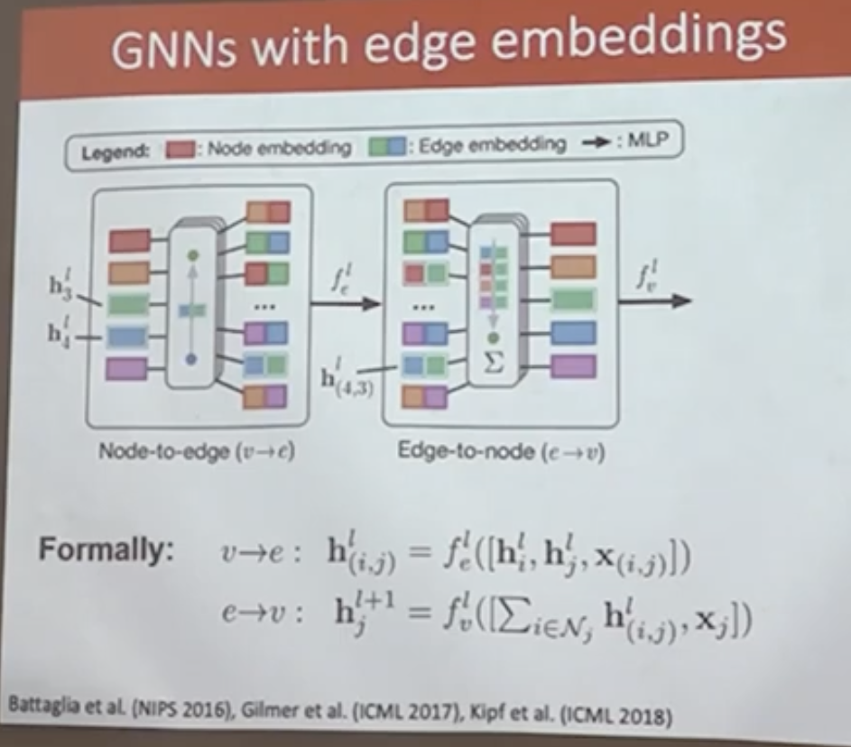
Graph Neural Networks with Edge Embeddings#
In many graph-structured problems, edges carry rich information that cannot be captured by the adjacency matrix alone. Examples include bond types in molecular graphs, relationship types in knowledge graphs, or distances and weights in physical networks. To incorporate such information, Graph Neural Networks can be extended to explicitly learn edge embeddings alongside node embeddings.
A common approach alternates between two message-passing steps:
Node-to-edge update \( (v \rightarrow e)\)#
Each edge embedding is updated using the embeddings of its incident nodes together with the edge features:
where \( \mathbf{h}_i \) and \( \mathbf{h}_j \) are node embeddings, \( \mathbf{x}_{(i,j)} \) denotes edge attributes, and \( f_e \) is a learnable function (typically a multilayer perceptron).
Edge-to-node update \((e \rightarrow v)\)#
Node embeddings are updated by aggregating messages from incident edges:
where the aggregation operator is permutation invariant and \( f_v \) is another learnable function.
This alternating update scheme preserves permutation equivariance at the node level while enabling the model to capture rich interactions between nodes and edges. Such architectures form the foundation of message-passing neural networks and are widely used in molecular modeling, physical simulation, and relational reasoning tasks.
Image(filename='images/GNN_edgeemb.png', width=700)
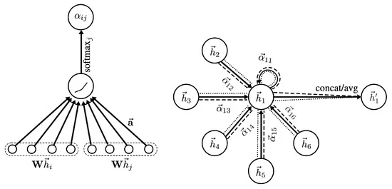
Graph Neural Network with attention#
In Graph Neural Networks, a central operation is the aggregation of information from the neighbors of a node. A simple approach is to aggregate neighbor embeddings using sum or average pooling. While these operators are permutation invariant and can handle a variable number of neighbors, they assign equal importance to all neighboring nodes.
More expressive aggregation mechanisms can also be considered. For instance, sequence-based models such as LSTMs are capable of processing a variable number of neighbors. However, such models are not permutation invariant and therefore depend on an arbitrary ordering of the neighbors. Since graphs do not admit a canonical ordering of nodes, this makes sequence-based aggregation unsuitable for general graph-structured data.
A principled and effective alternative is \emph{attention-based aggregation}. Attention mechanisms allow the model to learn adaptive importance weights for different neighbors while preserving permutation invariance. Instead of treating all neighbors equally, the model learns to focus on the most relevant ones.
Attention-based aggregation provides a principled solution to this problem. Attention mechanisms allow the model to learn adaptive, data-driven weights that quantify the importance of each neighbor while preserving permutation invariance.
Single-head attention.#
In attention-based GNNs, two distinct sets of parameters are learned: (i) a weight matrix that transforms node embeddings, and (ii) a separate attention mechanism that models pairwise interactions between neighboring nodes.
First, node embeddings are linearly transformed: $\( \mathbf{z}_i = \mathbf{W}\,\mathbf{h}_i, \)\( where \)\mathbf{W}$ is a learnable weight matrix shared across all nodes.
Next, for each edge \((i,j)\), an unnormalized attention score is computed using a learnable interaction function: $\( e_{ij} = \text{LeakyReLU} \left( \mathbf{a}^{\top} \left[ \mathbf{z}_i \,\Vert\, \mathbf{z}_j \right] \right), \)\( where \)\mathbf{a}\( is a learnable attention vector and \)[\cdot \Vert \cdot]$ denotes concatenation.
The attention coefficients are obtained via softmax normalization over the neighborhood: $\( a_{ij} = \frac{\exp(e_{ij})} {\sum_{k \in \mathcal{N}_i} \exp(e_{ik})}. \)$
Finally, the updated node embedding is computed as an attention-weighted aggregation of transformed neighbor embeddings: $\( \mathbf{h}_i^{(l+1)} = \sum_{j \in \mathcal{N}_i} a_{ij}\,\mathbf{z}_j. \)$
This formulation preserves permutation invariance while allowing the model to focus on the most informative neighbors.
Multi-head attention.#
To stabilize training and increase representational capacity, multiple independent attention heads are often employed. For each head \(k \in \{1,\dots,K\}\), separate parameters \(\mathbf{W}^k\) and \(\mathbf{a}^k\) are learned.
The output of the multi-head attention layer is given by $\( \mathbf{h}_i^{(l+1)} = \sigma \left( \frac{1}{K} \sum_{k=1}^{K} \sum_{j \in \mathcal{N}_i} a_{ij}^{k}\, \mathbf{W}^{k}\mathbf{h}_j \right), \)\( where \)a_{ij}^{k}\( denotes the attention coefficient computed by head \)k\(, and \)\sigma(\cdot)$ is a nonlinear activation function.
Multi-head attention enables the model to attend to different aspects of the neighborhood simultaneously, leading to more expressive and robust node representations.
Image(filename='images/GNN_atten.jpg', width=700)
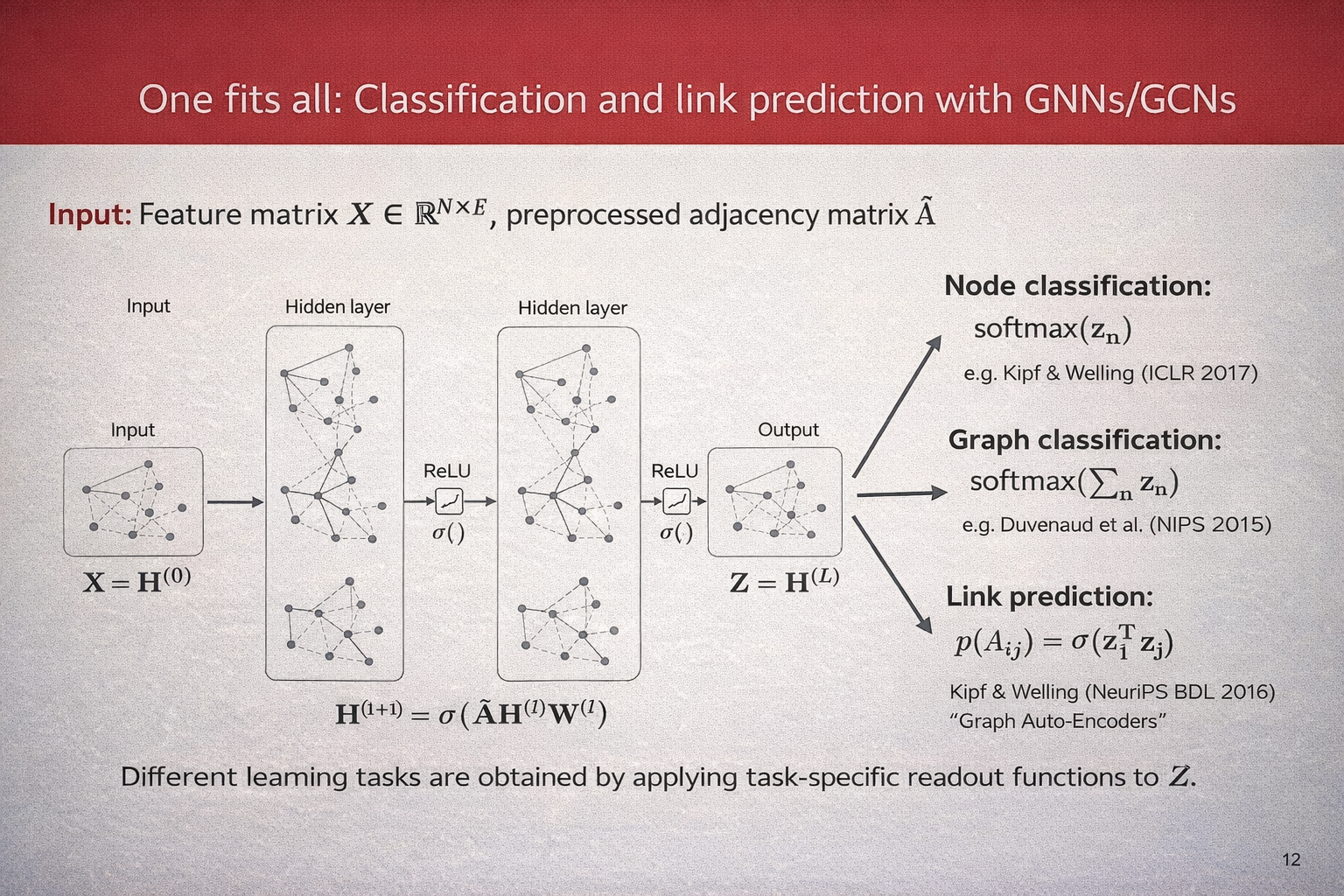
A Unified View: Classification and Link Prediction with GNNs#
Graph Neural Networks provide a unified framework for a wide range of learning tasks on graphs. Given a graph with \(N\) nodes, let $\( \mathbf{X} \in \mathbb{R}^{N \times F} \)\( denote the node feature matrix and let \)\hat{\mathbf{A}}$ be the preprocessed adjacency matrix (including self-loops and normalization).
A GNN (or GCN) computes a sequence of hidden representations by repeatedly applying a message-passing layer of the form $\( \mathbf{H}^{(l+1)} = \sigma\!\left(\hat{\mathbf{A}}\,\mathbf{H}^{(l)}\mathbf{W}^{(l)}\right), \)\( where \)\mathbf{H}^{(0)} = \mathbf{X}\(, \)\mathbf{W}^{(l)}\( are learnable weight matrices, and \)\sigma(\cdot)\( is a nonlinear activation function. After \)L\( layers, we obtain the final node embeddings \)\( \mathbf{Z} = \mathbf{H}^{(L)}. \)$
Different learning tasks are obtained by applying task-specific readout functions to \(\mathbf{Z}\).
\paragraph{Node classification.} For node-level prediction, a classifier is applied independently to each node embedding: $\( p(y_n \mid \mathbf{Z}) = \text{softmax}(\mathbf{z}_n), \)\( where \)\mathbf{z}_n\( denotes the embedding of node \)n$. This setting is commonly used in semi-supervised learning on graphs.
\paragraph{Graph classification.} For graph-level prediction, node embeddings are aggregated into a single graph representation using a permutation-invariant pooling operation, such as summation: $\( \mathbf{z}_G = \sum_{n=1}^{N} \mathbf{z}_n, \)\( followed by a classifier: \)\( p(y_G \mid \mathbf{Z}) = \text{softmax}(\mathbf{z}_G). \)$
\paragraph{Link prediction.} For link prediction, node embeddings are used to estimate the probability of an edge between two nodes. A common choice is an inner-product decoder: $\( p(A_{ij} = 1 \mid \mathbf{Z}) = \sigma\!\left(\mathbf{z}_i^{\top}\mathbf{z}_j\right), \)\( where \)\sigma(\cdot)$ denotes the logistic sigmoid function.
This formulation highlights that a single GNN encoder can be reused across multiple tasks, with only the output layer or readout function changing depending on the learning objective.
Image(filename='images/GNN_overview.png', width=700)
Smoothness in Graph Neural Networks#
A fundamental assumption underlying Graph Neural Networks is the principle of \emph{smoothness} on graphs. Smoothness expresses the idea that nodes that are close or strongly connected in the graph structure are likely to have similar representations and labels.
Intuition.#
In many real-world graphs, such as social networks, citation networks, or molecular graphs, neighboring nodes often share semantic or functional similarity. Graph Neural Networks exploit this assumption by propagating and averaging information across edges, thereby encouraging neighboring nodes to have similar embeddings.
Smoothness via message passing.#
Consider a generic GCN layer of the form $\( \mathbf{H}^{(l+1)} = \sigma\!\left(\hat{\mathbf{A}}\,\mathbf{H}^{(l)}\mathbf{W}^{(l)}\right), \)\( where \)\hat{\mathbf{A}}\( is the normalized adjacency matrix. Multiplication by \)\hat{\mathbf{A}}$ performs a local averaging of node representations over the graph neighborhood. As a result, node embeddings become progressively smoother across edges as the number of layers increases.
Connection to graph Laplacian regularization.#
The smoothness assumption can be formalized using the graph Laplacian. Let \(\mathbf{Z} \in \mathbb{R}^{N \times d}\) denote the matrix of node embeddings. A common smoothness regularizer is $\( \mathcal{R}_{\text{smooth}}(\mathbf{Z}) = \frac{1}{2} \sum_{i,j} A_{ij} \lVert \mathbf{z}_i - \mathbf{z}_j \rVert^2 =\mathrm{Tr}\!\left(\mathbf{Z}^{\top}\mathbf{L}\mathbf{Z}\right), \)\( where \)\mathbf{L} = \mathbf{D} - \mathbf{A}$ is the graph Laplacian. Minimizing this term explicitly enforces similar embeddings for neighboring nodes.
GCN layers can be interpreted as implicitly minimizing such a smoothness objective, thereby acting as a form of Laplacian regularization.
Benefits and limitations.#
Smoothness is a powerful inductive bias that enables effective semi-supervised learning and label propagation on graphs. However, excessive smoothing can be detrimental. As multiple GNN layers are stacked, node embeddings may converge to similar values across the graph, a phenomenon known as \emph{over-smoothing}.
\paragraph{Over-smoothing.} Over-smoothing occurs when repeated neighborhood aggregation causes node embeddings to become indistinguishable: $\( \mathbf{z}_i \approx \mathbf{z}_j \quad \forall i,j. \)$ This limits the expressive power of deep GNNs and degrades performance on tasks that require discriminative node representations.
Mitigation strategies. Common techniques to mitigate over-smoothing include:
limiting the depth of GNNs,
residual or skip connections,
normalization and regularization techniques,
attention mechanisms that adaptively weight neighbors.
Overall, smoothness provides a crucial theoretical foundation for Graph Neural Networks, explaining both their strengths in relational learning and their limitations when applied too aggressively.
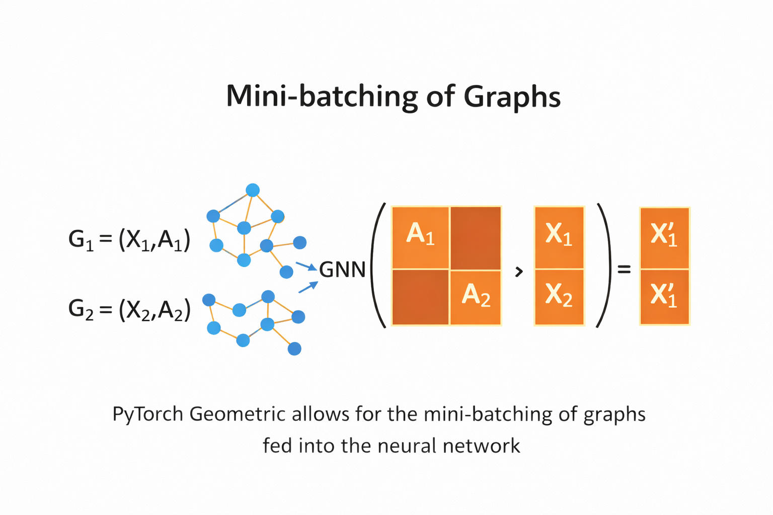
Mini-batching and Training Strategies for Graph Neural Networks#
Unlike standard deep learning models, Graph Neural Networks operate on structured data with dependencies between nodes. As a result, constructing mini-batches for training is non-trivial and requires special care. Several batching strategies have been proposed, each with different trade-offs in terms of scalability, memory usage, and approximation quality.
Full-batch training.#
The simplest approach is full-batch training, where the entire graph is processed at once: $\( \mathbf{H}^{(l+1)} = \sigma\!\left(\hat{\mathbf{A}}\,\mathbf{H}^{(l)}\mathbf{W}^{(l)}\right). \)$ This approach preserves exact message passing and is commonly used in semi-supervised node classification on small graphs. However, it does not scale to large graphs due to memory and computational constraints.
Graph-level mini-batching.#
For graph classification tasks, the dataset typically consists of many small, independent graphs. In this setting, mini-batching is straightforward: multiple graphs are combined into a batch by constructing a block-diagonal adjacency matrix: $\( \hat{\mathbf{A}}_{\text{batch}} = \begin{bmatrix} \hat{\mathbf{A}}^{(1)} & 0 & \cdots & 0 \\ 0 & \hat{\mathbf{A}}^{(2)} & \cdots & 0 \\ \vdots & \vdots & \ddots & \vdots \\ 0 & 0 & \cdots & \hat{\mathbf{A}}^{(B)} \end{bmatrix}. \)$ This allows standard mini-batch training while preserving graph independence and permutation invariance.
Node-wise mini-batching with neighbor sampling.#
For large single-graph settings, node-wise mini-batching is commonly employed. A subset of target nodes is sampled, and only a fixed number of neighbors is expanded at each layer. For a \(L\)-layer GNN, this produces a computation graph of bounded size: $\( \mathcal{B}^{(l)} = \bigcup_{i \in \mathcal{B}^{(l+1)}} \mathcal{S}_l(i), \)\( where \)\mathcal{S}_l(i)\( denotes the sampled neighbors of node \)i\( at layer \)l$. This strategy reduces memory usage but introduces stochasticity and approximation error.
\paragraph{Layer-wise sampling.} An alternative is layer-wise sampling, where a fixed set of nodes is sampled per layer rather than per target node. This approach avoids the exponential neighborhood expansion common in node-wise sampling and improves scalability for deep GNNs.
Subgraph-based mini-batching.#
Another approach is to sample induced subgraphs from the original graph and treat each subgraph as a mini-batch. Message passing is performed only within the sampled subgraph: $\( \mathbf{H}_{\mathcal{S}}^{(l+1)} = \sigma\!\left(\hat{\mathbf{A}}_{\mathcal{S}}\,\mathbf{H}_{\mathcal{S}}^{(l)}\mathbf{W}^{(l)}\right), \)\( where \)\mathcal{S}$ denotes the sampled node set. This method preserves local structure while enabling scalable training.
Trade-offs.#
Each batching strategy involves trade-offs between accuracy and efficiency:
Full-batch training is exact but does not scale.
Graph-level batching is efficient but limited to independent graphs.
Sampling-based methods scale to large graphs but introduce bias and variance.
Selecting an appropriate batching strategy depends on the task, graph size, and available computational resources.
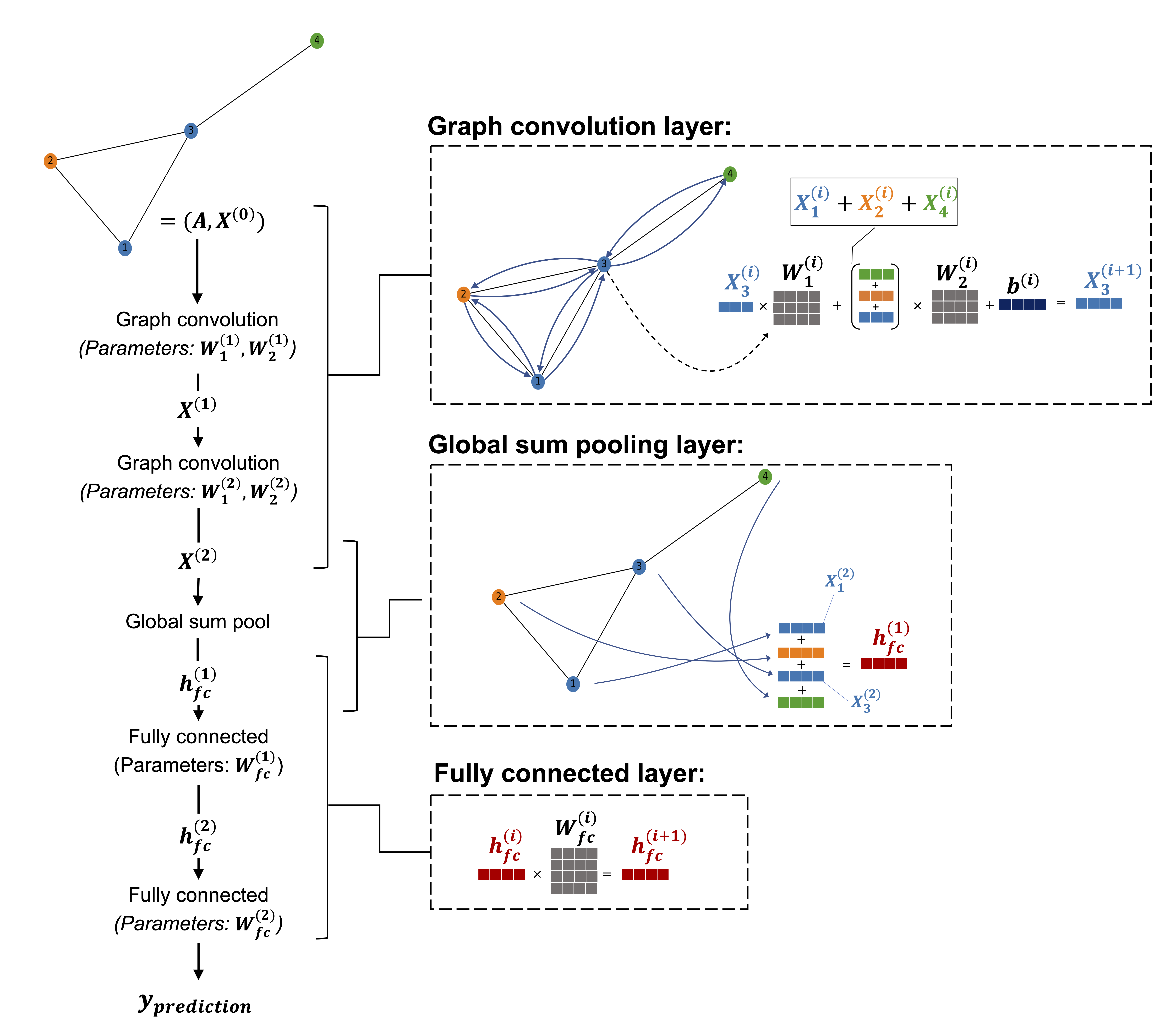
Implementing a GNN in PyTorch from scratch#
Defining the NodeNetwork model#
import networkx as nx
import torch
from torch.nn.parameter import Parameter
import numpy as np
import torch.nn.functional as F
class NodeNetwork(torch.nn.Module):

    def __init__(self, input_features):
        super().__init__()

        self.conv_1 = BasicGraphConvolutionLayer(input_features, 32)
        self.conv_2 = BasicGraphConvolutionLayer(32, 32)
        self.fc_1 = torch.nn.Linear(32, 16)
        self.out_layer = torch.nn.Linear(16, 2)

    def forward(self, X, A,batch_mat):
        x = self.conv_1(X, A).clamp(0)
        x = self.conv_2(x, A).clamp(0)
        output = global_sum_pool(x, batch_mat)
        output = self.fc_1(output)
        output = self.out_layer(output)
        return F.softmax(output, dim=1)
The NodeNetwork’s graph convolution layer#
class BasicGraphConvolutionLayer(torch.nn.Module):

    def __init__(self, in_channels, out_channels):
        super().__init__()
        self.in_channels = in_channels
        self.out_channels = out_channels

        self.W2 = Parameter(torch.rand(
             (in_channels, out_channels), dtype=torch.float32))
        self.W1 = Parameter(torch.rand(
             (in_channels, out_channels), dtype=torch.float32))

        self.bias = Parameter(torch.zeros(
                 out_channels, dtype=torch.float32))

    def forward(self, X, A):
        potential_msgs = torch.mm(X, self.W2)
        propagated_msgs = torch.mm(A, potential_msgs)
        root_update = torch.mm(X, self.W1)
        output = propagated_msgs + root_update + self.bias
        return output
Adding a global pooling layer to deal with varying graph sizes#
def global_sum_pool(X, batch_mat):
    if batch_mat is None or batch_mat.dim() == 1:
        return torch.sum(X, dim=0).unsqueeze(0)
    else:
        return torch.mm(batch_mat, X)
Image(filename='figures/18_10.png', width=600)
---------------------------------------------------------------------------
FileNotFoundError                         Traceback (most recent call last)
Cell In[20], line 1
----> 1 Image(filename='figures/18_10.png', width=600)

File ~/miniforge3/envs/jupyterbook/lib/python3.10/site-packages/IPython/core/display.py:1053, in Image.__init__(self, data, url, filename, format, embed, width, height, retina, unconfined, metadata, alt)
   1051 self.unconfined = unconfined
   1052 self.alt = alt
-> 1053 super(Image, self).__init__(data=data, url=url, filename=filename,
   1054         metadata=metadata)
   1056 if self.width is None and self.metadata.get('width', {}):
   1057     self.width = metadata['width']

File ~/miniforge3/envs/jupyterbook/lib/python3.10/site-packages/IPython/core/display.py:371, in DisplayObject.__init__(self, data, url, filename, metadata)
    368 elif self.metadata is None:
    369     self.metadata = {}
--> 371 self.reload()
    372 self._check_data()

File ~/miniforge3/envs/jupyterbook/lib/python3.10/site-packages/IPython/core/display.py:1088, in Image.reload(self)
   1086 """Reload the raw data from file or URL."""
   1087 if self.embed:
-> 1088     super(Image,self).reload()
   1089     if self.retina:
   1090         self._retina_shape()

File ~/miniforge3/envs/jupyterbook/lib/python3.10/site-packages/IPython/core/display.py:397, in DisplayObject.reload(self)
    395 if self.filename is not None:
    396     encoding = None if "b" in self._read_flags else "utf-8"
--> 397     with open(self.filename, self._read_flags, encoding=encoding) as f:
    398         self.data = f.read()
    399 elif self.url is not None:
    400     # Deferred import

FileNotFoundError: [Errno 2] No such file or directory: 'figures/18_10.png'
def get_batch_tensor(graph_sizes):
    starts = [sum(graph_sizes[:idx]) for idx in range(len(graph_sizes))]
    stops = [starts[idx]+graph_sizes[idx] for idx in range(len(graph_sizes))]
    tot_len = sum(graph_sizes)
    batch_size = len(graph_sizes)
    batch_mat = torch.zeros([batch_size, tot_len]).float()
    for idx, starts_and_stops in enumerate(zip(starts, stops)):
        start = starts_and_stops[0]
        stop = starts_and_stops[1]
        batch_mat[idx, start:stop] = 1
    return batch_mat
def collate_graphs(batch):
    adj_mats = [graph['A'] for graph in batch]
    sizes = [A.size(0) for A in adj_mats]
    tot_size = sum(sizes)
    # create batch matrix
    batch_mat = get_batch_tensor(sizes)
    # combine feature matrices
    feat_mats = torch.cat([graph['X'] for graph in batch],dim=0)
    # combine labels
    labels = torch.cat([graph['y'] for graph in batch], dim=0)
    # combine adjacency matrices
    batch_adj = torch.zeros([tot_size, tot_size], dtype=torch.float32)
    accum = 0
    for adj in adj_mats:
        g_size = adj.shape[0]
        batch_adj[accum:accum+g_size, accum:accum+g_size] = adj
        accum = accum + g_size
    repr_and_label = {
            'A': batch_adj,
            'X': feat_mats,
            'y': labels,
            'batch' : batch_mat}

    return repr_and_label
Preparing the DataLoader#
def get_graph_dict(G, mapping_dict):
    # build dictionary representation of graph G
    A = torch.from_numpy(np.asarray(nx.adjacency_matrix(G).todense())).float()
    # build_graph_color_label_representation() was introduced with the first example graph
    X = torch.from_numpy(build_graph_color_label_representation(G,mapping_dict)).float()
    # kludge since there is not specific task for this example
    y = torch.tensor([[1, 0]]).float()
    return {'A': A, 'X': X, 'y': y, 'batch': None}

# building 4 graphs to treat as a dataset

blue, orange, green = "#1f77b4", "#ff7f0e","#2ca02c"
mapping_dict = {green: 0, blue: 1, orange: 2}

G1 = nx.Graph()
G1.add_nodes_from([(1, {"color": blue}),
                   (2, {"color": orange}),
                   (3, {"color": blue}),
                   (4, {"color": green})])
G1.add_edges_from([(1, 2), (2, 3),(1, 3), (3, 4)])
G2 = nx.Graph()
G2.add_nodes_from([(1, {"color": green}),
                   (2, {"color": green}),
                   (3, {"color": orange}),
                   (4, {"color": orange}),
                   (5,{"color": blue})])
G2.add_edges_from([(2, 3),(3, 4),(3, 1),(5, 1)])
G3 = nx.Graph()
G3.add_nodes_from([(1, {"color": orange}),
                   (2, {"color": orange}),
                   (3, {"color": green}),
                   (4, {"color": green}),
                   (5, {"color": blue}),
                   (6, {"color":orange})])
G3.add_edges_from([(2, 3), (3, 4), (3, 1), (5, 1), (2, 5), (6, 1)])
G4 = nx.Graph()
G4.add_nodes_from([(1, {"color": blue}), (2, {"color": blue}), (3, {"color": green})])
G4.add_edges_from([(1, 2), (2, 3)])
graph_list = [get_graph_dict(graph,mapping_dict) for graph in [G1, G2, G3, G4]]
Image(filename='figures/18_11.png', width=600)
from torch.utils.data import Dataset
from torch.utils.data import DataLoader


class ExampleDataset(Dataset):

    # Simple PyTorch dataset that will use our list of graphs
    def __init__(self, graph_list):
        self.graphs = graph_list

    def __len__(self):
        return len(self.graphs)

    def __getitem__(self,idx):
        mol_rep = self.graphs[idx]
        return mol_rep
dset = ExampleDataset(graph_list)
# Note how we use our custom collate function
loader = DataLoader(dset, batch_size=2, shuffle=False, collate_fn=collate_graphs)
Using the NodeNetwork to make predictions#
torch.manual_seed(123)
node_features = 3
net = NodeNetwork(node_features)
batch_results = []

for b in loader:
    batch_results.append(net(b['X'], b['A'], b['batch']).detach())

G1_rep = dset[1]
G1_single = net(G1_rep['X'], G1_rep['A'], G1_rep['batch']).detach()

G1_batch = batch_results[0][1]
torch.all(torch.isclose(G1_single, G1_batch))
Example: Node classification in citation network#
The Cora dataset is a benchmark citation network widely used in graph machine learning and graph neural network research. It consists of 2,708 nodes representing scientific publications and 5,429 edges denoting citation relationships between papers. Each node is described by a 1,433-dimensional binary feature vector indicating the presence or absence of specific words in the paper, and each node belongs to one of seven research topic classes. The dataset is provided as a single, fixed graph with predefined training, validation, and test splits, making it especially suitable for semi-supervised node classification tasks. Cora is commonly used to evaluate algorithms such as Graph Convolutional Networks (GCNs) due to its moderate size, sparse structure, and well-understood characteristics. In the PyTorch Geometric Planetoid version of the Cora dataset, node features are provided as indexed binary vectors without explicit names, although each feature actually corresponds to the presence of a specific word from the original paper vocabulary.
from torch_geometric.datasets import Planetoid
from torch_geometric.transforms import NormalizeFeatures

cora_dataset = Planetoid(root="Cora_data", name="Cora", transform=NormalizeFeatures())
print(len(cora_dataset))
data = cora_dataset[0]
print(cora_dataset)
print(data)
1
Cora()
Data(x=[2708, 1433], edge_index=[2, 10556], y=[2708], train_mask=[2708], val_mask=[2708], test_mask=[2708])
# ===== Cora Dataset Inspection (PyTorch Geometric) =====
print("===== GRAPH SUMMARY =====")
print(data)
print()
print("===== BASIC STATISTICS =====")
print(f"Number of nodes: {data.num_nodes}")
print(f"Number of edges: {data.num_edges}")
print(f"Average node degree: {data.num_edges / data.num_nodes:.2f}")
print(f"Is undirected: {data.is_undirected()}")
print(f"Number of Feature: {data.num_features}")
print()
print("===== NODE FEATURES =====")
print(f"Feature matrix shape: {data.x.shape}")
print(f"Number of node features: {cora_dataset.num_node_features}")
print(f"First node feature vector:\n{data.x[0]}")
print()
print("===== LABELS =====")
print(f"Label tensor shape: {data.y.shape}")
print(f"Number of classes: {cora_dataset.num_classes}")
print()
print("===== DATA SPLITS =====")
print(f"Training nodes: {int(data.train_mask.sum())}")
print(f"Validation nodes: {int(data.val_mask.sum())}")
print(f"Test nodes: {int(data.test_mask.sum())}")
print()
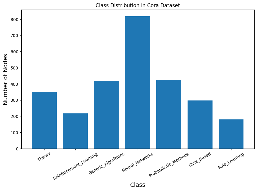
print("===== CLASS DISTRIBUTION =====")
for c in range(cora_dataset.num_classes):
count = int((data.y == c).sum())
print(f"Class {c}: {count} nodes")
print()
print("===== EDGE INFORMATION =====")
print(f"Edge index shape: {data.edge_index.shape}")
print("First 10 edges:")
print(data.edge_index[:, :10])
===== GRAPH SUMMARY =====
Data(x=[2708, 1433], edge_index=[2, 10556], y=[2708], train_mask=[2708], val_mask=[2708], test_mask=[2708])

===== BASIC STATISTICS =====
Number of nodes: 2708
Number of edges: 10556
Average node degree: 3.90
Is undirected: True
Number of Feature: 1433

===== NODE FEATURES =====
Feature matrix shape: torch.Size([2708, 1433])
Number of node features: 1433
First node feature vector:
tensor([0., 0., 0.,  ..., 0., 0., 0.])

===== LABELS =====
Label tensor shape: torch.Size([2708])
Number of classes: 7

===== DATA SPLITS =====
Training nodes: 140
Validation nodes: 500
Test nodes: 1000

===== CLASS DISTRIBUTION =====
Class 0: 351 nodes
Class 1: 217 nodes
Class 2: 418 nodes
Class 3: 818 nodes
Class 4: 426 nodes
Class 5: 298 nodes
Class 6: 180 nodes

===== EDGE INFORMATION =====
Edge index shape: torch.Size([2, 10556])
First 10 edges:
tensor([[ 633, 1862, 2582,    2,  652,  654,    1,  332, 1454, 1666],
        [   0,    0,    0,    1,    1,    1,    2,    2,    2,    2]])
Manual label mapping based on original Cora dataset documentation#
Note: PyTorch Geometric does not expose the official label-name mapping
label_dict = {
    0: "Theory",
    1: "Reinforcement_Learning",
    2: "Genetic_Algorithms",
    3: "Neural_Networks",
    4: "Probabilistic_Methods",
    5: "Case_Based",
    6: "Rule_Learning"
}
import collections
import matplotlib.pyplot as plt


# Count class occurrences
counter = collections.Counter(data.y.numpy())
counter = dict(counter)
print(counter)

# Sort by class index
classes = sorted(counter.keys())
counts = [counter[c] for c in classes]
labels = [label_dict[c] for c in classes]

# Plot
plt.figure(figsize=(10, 6))
plt.bar(labels, counts)
plt.xlabel("Class", fontsize=14)
plt.ylabel("Number of Nodes", fontsize=14)
plt.xticks(rotation=30)
plt.title("Class Distribution in Cora Dataset")
plt.show()
{np.int64(3): 818, np.int64(4): 426, np.int64(0): 351, np.int64(2): 418, np.int64(1): 217, np.int64(5): 298, np.int64(6): 180}
import networkx as nx
import matplotlib.pyplot as plt
from torch_geometric.utils import to_networkx
# Color palette (one per class)
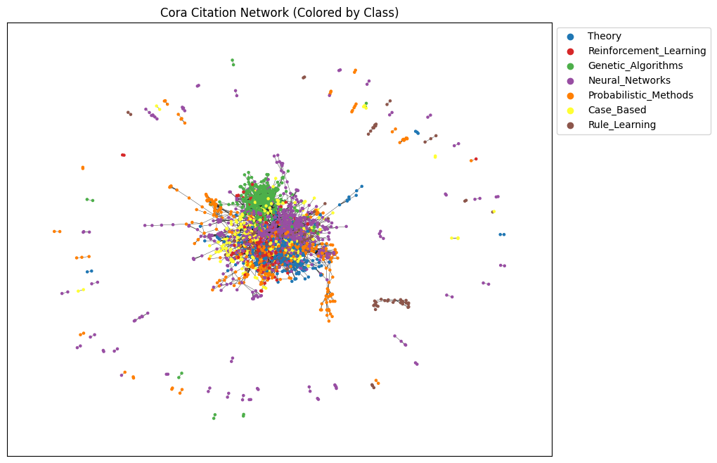
colorlist = [
"#1f77b4", "#d62728", "#4daf4a",
"#984ea3", "#ff7f00", "#ffff33", "#8c564b"
]
# Convert PyG graph to NetworkX graph
G = to_networkx(data, to_undirected=True)
# Assign node colors based on labels
node_colors = [colorlist[int(label)] for label in data.y]
# Layout
pos = nx.spring_layout(G, seed=42)
# Prepare node colors
node_colors = [colorlist[int(label)] for label in data.y]
# Layout
pos = nx.spring_layout(G, seed=42)
plt.figure(figsize=(10, 8))
nx.draw_networkx_nodes(G, pos, node_size=5, node_color=node_colors)
nx.draw_networkx_edges(G, pos, width=0.25)
# Legend (explicit index-based mapping)
for i in range(len(label_dict)):
plt.scatter([], [], c=colorlist[i], label=label_dict[i])
plt.legend(bbox_to_anchor=(1, 1), loc="upper left")
plt.title("Cora Citation Network (Colored by Class)")
plt.show()
Two-layer Graph Convolutional Network (GCN)#
The follwoing two-layer Graph Convolutional Network (GCN) takes node features and graph connectivity as input, learns hidden node representations through neighborhood aggregation, and outputs class logits for each node, where the number of output channels corresponds to the number of target classes in the dataset.
The GCN class defines a simple two-layer Graph Convolutional Network used for node classification on graph-structured data such as the Cora citation network. The __init__ method initializes the model by setting a fixed random seed for reproducibility and defining two graph convolution layers: the first layer (conv1) transforms the input node features into a lower-dimensional hidden representation, while the second layer (conv2) maps these hidden representations to the final output space, whose size equals the number of target classes. In the forward method, the model receives a graph object containing node features (x) and edge information (edge_index), applies the first graph convolution followed by a ReLU activation to introduce non-linearity, and then uses dropout to reduce overfitting during training. Finally, the second graph convolution produces a matrix of output scores (logits) for each node, which are later used with a loss function such as cross-entropy to train the model for node classification.
import torch
import torch.nn as nn
import torch.nn.functional as F
from torch_geometric.nn import GCNConv

class GCN(nn.Module):
    def __init__(self, input_channels, output_channels, hidden_channels=16):
        super().__init__()
        torch.manual_seed(123)

        self.conv1 = GCNConv(in_channels=input_channels, out_channels=hidden_channels)
        self.conv2 = GCNConv(in_channels=hidden_channels, out_channels=output_channels)

    def forward(self, data):
        x, edge_index = data.x, data.edge_index

        x = self.conv1(x, edge_index)
        x = x.relu()
        x = F.dropout(x, p=0.5, training=self.training)

        x = self.conv2(x, edge_index)
        return x

model = GCN(
    input_channels=cora_dataset.num_node_features,
    output_channels=cora_dataset.num_classes,
    hidden_channels=16
)
print(model)
GCN(
  (conv1): GCNConv(1433, 16)
  (conv2): GCNConv(16, 7)
)
model.eval()
with torch.no_grad():
    out = model(data)

print("out:", out.shape, out.dtype, out.device)
print("labels:", data.y.shape, data.y.dtype, data.y.device)
out: torch.Size([2708, 7]) torch.float32 cpu
labels: torch.Size([2708]) torch.int64 cpu
import os
os.environ["OMP_NUM_THREADS"] = "1"
os.environ["MKL_NUM_THREADS"] = "1"
import numpy as np
import matplotlib.pyplot as plt
from sklearn.manifold import TSNE
import torch
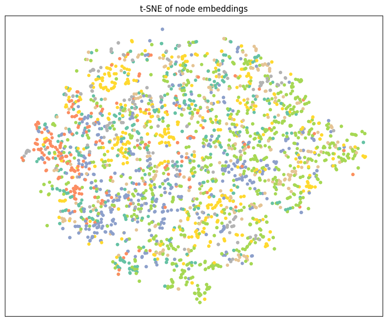
def visualize_tsne(emb, labels, seed=42):
X = emb.detach().cpu().numpy().astype(np.float32)
y = labels.detach().cpu().numpy()
n = X.shape[0]
perplexity = min(30, max(5, (n - 1) // 3))
tsne = TSNE(
n_components=2,
init="pca",
learning_rate="auto",
perplexity=perplexity,
random_state=seed,
method="barnes_hut",
angle=0.5
)
Z = tsne.fit_transform(X)
plt.figure(figsize=(10, 8))
plt.xticks([])
plt.yticks([])
plt.scatter(Z[:, 0], Z[:, 1], s=15, c=y, cmap="Set2")
plt.title("t-SNE of node embeddings")
plt.show()
# Run safely
model.eval()
with torch.no_grad():
out = model(data)
visualize_tsne(out, data.y)
The following code initializes the main components required to train a Graph Convolutional Network (GCN) for node classification. First, the GCN model is created by specifying the number of input channels (equal to the number of node features) and output channels (equal to the number of classes), and then moved to the chosen computation device (CPU or GPU) using .to(device). Next, the Adam optimizer is defined, which updates the model parameters during training; the learning rate controls how large each update step is, while weight decay acts as a regularization term to reduce overfitting. Finally, the loss function is set to CrossEntropyLoss, which is the standard choice for multi-class classification problems and compares the model’s predicted class scores (logits) with the true node labels. Together, these components prepare the model for the training loop, where the optimizer minimizes the loss by adjusting the GCN’s weights.
import torch
import torch.nn as nn

# input_channels = dataset.num_node_features
# output_channels = dataset.num_classes
# device = torch.device("cuda" if torch.cuda.is_available() else "cpu")

model = GCN(
    input_channels=cora_dataset.num_node_features,
    output_channels=cora_dataset.num_classes,
    hidden_channels=16)
optimizer = torch.optim.Adam(
    model.parameters(),
    lr=0.01,
    weight_decay=5e-4
)

criterion = nn.CrossEntropyLoss()
The following code implements the training loop for a Graph Convolutional Network (GCN) on the Cora dataset. First, the number of training epochs is set, which determines how many times the model will see the entire graph during training. The graph data is then moved to the chosen device (CPU or GPU) so that computations are performed consistently.
Inside the loop, model.train() puts the network in training mode, enabling behaviors such as dropout. At the start of each epoch, existing gradients are cleared using optimizer.zero_grad() to prevent accumulation from previous updates. The model then performs a forward pass on the full graph, producing class scores for every node.
The loss is computed only on the training nodes using train_mask, which is important in semi-supervised learning because labels are available for only a subset of nodes. After computing the loss, loss.backward() calculates gradients with respect to the model parameters, and optimizer.step() updates those parameters to reduce the loss.
Finally, the code calculates training accuracy by comparing the predicted class of each training node with its true label. Printing the loss and accuracy every few epochs allows students to monitor whether the model is learning and improving over time.
# Training settings
num_epochs = 200

# Move graph to device
cora_graph = cora_dataset[0]

for epoch in range(num_epochs):
    model.train()

    # Reset gradients
    optimizer.zero_grad()

    # Forward pass
    out = model(cora_graph)

    # Compute loss on training nodes only
    loss = criterion(
        out[cora_graph.train_mask],
        cora_graph.y[cora_graph.train_mask]
    )

    # Backpropagation
    loss.backward()
    optimizer.step()

    # Training accuracy
    pred_train = out.argmax(dim=1)
    correct_train = (
        pred_train[cora_graph.train_mask]
        == cora_graph.y[cora_graph.train_mask]
    ).sum()

    acc_train = int(correct_train) / int(cora_graph.train_mask.sum())

    # Print progress
    if epoch % 10 == 0:
        print(
            f"Epoch {epoch:03d} | "
            f"Loss: {loss.item():.4f} | "
            f"Train Accuracy: {acc_train:.4f}"
        )
The following code evaluates the trained Graph Convolutional Network on the test portion of the dataset, which contains nodes that were not used during training. The call to model.eval() puts the network into evaluation mode, ensuring that layers such as dropout behave correctly and do not introduce randomness during testing.
The with torch.no_grad(): block tells PyTorch not to compute gradients, which saves memory and speeds up execution since the model parameters are not being updated. The model then produces output scores for each node, and argmax(dim=1) selects the most likely class for every node.
To fairly measure performance, the code uses the test_mask to compare predictions only on test nodes, ignoring training and validation nodes. The number of correct predictions is divided by the total number of test nodes to compute the test accuracy, which reflects how well the model generalizes to unseen data.
# Switch model to evaluation mode
model.eval()

# Disable gradient computation for efficiency
with torch.no_grad():
    # Forward pass and predicted class labels
    pred = model(data).argmax(dim=1)

    # Count correct predictions on test nodes only
    correct = (
        pred[data.test_mask]
        == cora_graph.y[data.test_mask]
    ).sum().item()

    # Compute test accuracy
    test_acc = correct / data.test_mask.sum().item()

# Print test accuracy
print(f"Test Accuracy: {test_acc:.4f}")
import torch
import torch.nn as nn

# Create the GCN model
model = GCN(
    input_channels=cora_dataset.num_node_features,
    output_channels=cora_dataset.num_classes,
)

# Define the optimizer
optimizer = torch.optim.Adam(
    model.parameters(),
    lr=0.01,
    weight_decay=5e-4
)

# Define the loss function
criterion = nn.CrossEntropyLoss()
The following code extends the basic training loop by adding validation monitoring and best model selection, which are essential practices in machine learning. During each epoch, the model is first trained using only the nodes indicated by train_mask, and the loss is computed and minimized using backpropagation. Training accuracy is calculated to show how well the model fits the labeled training nodes.
After training in each epoch, the model is switched to evaluation mode to compute validation accuracy using val_mask. Validation nodes are not used for learning; instead, they provide an unbiased way to measure how well the model generalizes during training. By comparing validation accuracy across epochs, the code identifies when the model performs best on unseen data.
Whenever a new highest validation accuracy is achieved, the current model parameters are saved using a deep copy. After training finishes, the model is restored to this best-performing state. This approach helps prevent overfitting and ensures that the final model used for testing is the one that generalized best, not necessarily the one from the last training epoch
import copy

num_epochs = 200

# Track best validation accuracy and model
best_acc_val = 0.0
best_model_state = None

for epoch in range(num_epochs):
    # Training phase
    model.train()
    optimizer.zero_grad()

    out = model(cora_graph)

    loss = criterion(
        out[cora_graph.train_mask],
        cora_graph.y[cora_graph.train_mask]
    )
    loss.backward()
    optimizer.step()

    # Training accuracy
    pred_train = out.argmax(dim=1)
    correct_train = (
        pred_train[cora_graph.train_mask]
        == cora_graph.y[cora_graph.train_mask]
    ).sum()
    acc_train = int(correct_train) / int(cora_graph.train_mask.sum())

    # Validation phase
    model.eval()
    with torch.no_grad():
        out = model(cora_graph)
        pred_val = out.argmax(dim=1)

        correct_val = (
            pred_val[cora_graph.val_mask]
            == cora_graph.y[cora_graph.val_mask]
        ).sum()
        acc_val = int(correct_val) / int(cora_graph.val_mask.sum())

    # Save best model
    if acc_val > best_acc_val:
        best_acc_val = acc_val
        best_model_state = copy.deepcopy(model.state_dict())

    # Print progress
    if epoch % 10 == 0:
        print(
            f"Epoch {epoch:03d} | "
            f"Loss: {loss.item():.4f} | "
            f"Train Acc: {acc_train:.4f} | "
            f"Val Acc: {acc_val:.4f}"
        )

# Load best model after training
model.load_state_dict(best_model_state)
print(f"Best Validation Accuracy: {best_acc_val:.4f}")
import os
os.environ["OMP_NUM_THREADS"] = "1"
os.environ["MKL_NUM_THREADS"] = "1"

import numpy as np
import matplotlib.pyplot as plt
from sklearn.manifold import TSNE
import torch

def visualize_tsne(emb, labels, seed=42):
    X = emb.detach().cpu().numpy().astype(np.float32)
    y = labels.detach().cpu().numpy()

    n = X.shape[0]
    perplexity = min(30, max(5, (n - 1) // 3))

    tsne = TSNE(
        n_components=2,
        init="pca",
        learning_rate="auto",
        perplexity=perplexity,
        random_state=seed,
        method="barnes_hut",
        angle=0.5
    )

    Z = tsne.fit_transform(X)

    plt.figure(figsize=(10, 8))
    plt.xticks([])
    plt.yticks([])
    plt.scatter(Z[:, 0], Z[:, 1], s=15, c=y, cmap="Set2")
    plt.title("t-SNE of node embeddings")
    plt.show()

# Run safely
model.eval()
with torch.no_grad():
    out = model(data)

visualize_tsne(out, data.y)
# Load the best model obtained from validation
model.load_state_dict(best_model_state)

# Switch to evaluation mode
model.eval()

# ---- Test Accuracy ----
with torch.no_grad():
    pred = model(data).argmax(dim=1)

    correct = (
        pred[data.test_mask]
        == data.y[data.test_mask]
    ).sum().item()

    test_acc = correct / data.test_mask.sum().item()

print(f"Best Test Accuracy: {test_acc:.3f}")

# ---- Embedding Visualization ----
with torch.no_grad():
    out = model(data)

print("Node embedding shape:", out.shape)

# Visualize embeddings using true labels
visualize(out, color=data.y.cpu())
Example: Node classification using Graph Attention network#
This class defines a Graph Attention Network (GAT), which is a type of graph neural network that uses attention mechanisms to decide how important each neighboring node is during message passing.
The __init__ method sets up the model architecture. The first GATConv layer applies multi-head attention, meaning that multiple attention mechanisms operate in parallel to capture different aspects of neighborhood information. Each head learns how strongly a node should attend to its neighbors. The outputs of these heads are concatenated, which is why the input size of the second layer is hidden_channels × num_heads.
The second GATConv layer uses a single attention head and produces the final output, where each node receives a vector of length equal to the number of classes. This layer is typically used for node classification.
In the forward method, node features (x) and graph connectivity (edge_index) are extracted from the input graph. Dropout is applied to reduce overfitting. The first attention layer aggregates neighbor information using attention scores, followed by an ELU activation function to introduce nonlinearity. Another dropout layer is applied before the final attention layer, which outputs class scores for each node.
import torch
import torch.nn as nn
import torch.nn.functional as F
from torch_geometric.nn import GATConv


class GAT(torch.nn.Module):
    def __init__(
        self,
        input_channels,
        output_channels,
        hidden_channels=8,
        num_heads=8
    ):
        super().__init__()
        torch.manual_seed(123456)

        # First GAT layer with multi-head attention
        self.gatconv1 = GATConv(
            in_channels=input_channels,
            out_channels=hidden_channels,
            heads=num_heads
        )

        # Second GAT layer with a single attention head
        self.gatconv2 = GATConv(
            in_channels=hidden_channels * num_heads,
            out_channels=output_channels,
            heads=1
        )

    def forward(self, data):
        x, edge_index = data.x, data.edge_index

        # Dropout on input features
        x = F.dropout(x, p=0.6, training=self.training)

        # First GAT layer + nonlinearity
        x = self.gatconv1(x, edge_index)
        x = F.elu(x)

        # Dropout before final layer
        x = F.dropout(x, p=0.6, training=self.training)

        # Second GAT layer (output layer)
        x = self.gatconv2(x, edge_index)

        return x
import torch

# Select device (GPU if available, otherwise CPU)
device = torch.device("cuda" if torch.cuda.is_available() else "cpu")

# Load the Cora graph and move it to the selected device
cora_graph = cora_dataset[0].to(device)

# Define model input and output dimensions
input_channels = cora_dataset.num_features
output_channels = cora_dataset.num_classes

# Initialize the GCN model
model = GCN(
    input_channels=input_channels,
    output_channels=output_channels
).to(device)

# Print model architecture
print(model)

# Print total number of trainable parameters
print(
    "Number of parameters:",
    sum(p.numel() for p in model.parameters())
)
import matplotlib.pyplot as plt
from sklearn.manifold import TSNE

def visualize(h, color):
    # Reduce high-dimensional embeddings to 2D using t-SNE
    z = TSNE(n_components=2).fit_transform(
        h.detach().cpu().numpy()
    )

    # Plot settings
    plt.figure(figsize=(10, 8))
    plt.xticks([])
    plt.yticks([])

    # Scatter plot of nodes
    plt.scatter(
        z[:, 0],
        z[:, 1],
        s=70,
        c=color,
        cmap="Set2"
    )
    plt.show()


# Use the trained model to get node embeddings
model.eval()
out = model(cora_graph)

print("Node embedding shape:", out.shape)

# Visualize embeddings using true labels as colors
visualize(out, color=cora_graph.y.cpu())
import torch
import torch.nn as nn

# Initialize the GAT model
model = GAT(
    input_channels=input_channels,
    output_channels=output_channels
).to(device)

# Define optimizer
optimizer = torch.optim.Adam(
    model.parameters(),
    lr=0.005,
    weight_decay=5e-4
)

# Define loss function
criterion = nn.CrossEntropyLoss()


# ---------------- Training Loop ----------------
num_epochs = 200
cora_graph = cora_dataset[0].to(device)

for epoch in range(num_epochs):
    model.train()
    optimizer.zero_grad()

    # Forward pass
    out = model(cora_graph)

    # Compute loss on training nodes only
    loss = criterion(
        out[cora_graph.train_mask],
        cora_graph.y[cora_graph.train_mask]
    )

    # Backpropagation
    loss.backward()
    optimizer.step()
Training Accuracy + Progress Printing (Every 10 Epochs)#
# Get predictions on the training data
pred_train = out.argmax(dim=1)

# Count correct predictions only on training nodes
correct_train = (
    pred_train[cora_graph.train_mask]
    == cora_graph.y[cora_graph.train_mask]
).sum()

# Compute training accuracy
acc_train = int(correct_train) / int(cora_graph.train_mask.sum())

# Print training progress every 10 epochs
if (epoch + 1) % 10 == 0:
    print(
        f"Epoch: {epoch + 1:03d}, "
        f"Train Loss: {loss:.3f}, "
        f"Train Acc: {acc_train:.3f}"
    )
Testing the model#
# Set the model to evaluation mode
model.eval()

# Disable gradient computation for evaluation
with torch.no_grad():
    # Get predicted class labels for all nodes
    pred = model(cora_graph).argmax(dim=1)

    # Count correct predictions on test nodes only
    correct = (
        pred[cora_graph.test_mask]
        == cora_graph.y[cora_graph.test_mask]
    ).sum().item()

    # Compute test accuracy
    test_acc = correct / cora_graph.test_mask.sum().item()

# Print test accuracy
print(f"Test Accuracy: {test_acc:.4f}")
choose the best model based on validation data set#
%%time
import copy

num_epochs = 200

# Keep track of best validation accuracy and best model state
best_acc_val = 0.0
best_model_state = None

for epoch in range(num_epochs):

    # -------- TRAINING PHASE --------
    model.train()
    optimizer.zero_grad()

    out = model(cora_graph)

    # Training loss (only on training nodes)
    loss = criterion(
        out[cora_graph.train_mask],
        cora_graph.y[cora_graph.train_mask]
    )
    loss.backward()
    optimizer.step()

    # Training accuracy
    pred_train = out.argmax(dim=1)
    correct_train = (
        pred_train[cora_graph.train_mask]
        == cora_graph.y[cora_graph.train_mask]
    ).sum()
    acc_train = int(correct_train) / int(cora_graph.train_mask.sum())

    # -------- VALIDATION PHASE --------
    model.eval()
    with torch.no_grad():
        pred_val = model(cora_graph).argmax(dim=1)
        correct_val = (
            pred_val[cora_graph.val_mask]
            == cora_graph.y[cora_graph.val_mask]
        ).sum()
        acc_val = int(correct_val) / int(cora_graph.val_mask.sum())

    # -------- SAVE BEST MODEL --------
    if acc_val > best_acc_val:
        best_acc_val = acc_val
        best_model_state = copy.deepcopy(model.state_dict())

    # -------- LOGGING --------
    if (epoch + 1) % 10 == 0:
        print(
            f"Epoch: {epoch+1:03d}, "
            f"Train Loss: {loss:.3f}, "
            f"Train Acc: {acc_train:.3f}, "
            f"Val Acc: {acc_val:.3f}"
        )

# Load the best model after training
model.load_state_dict(best_model_state)
print(f"Best Validation Accuracy: {best_acc_val:.4f}")
Load Best Model, Test Accuracy, and Visualization#
# Print best validation accuracy and load best model
print("Best validation accuracy:", best_acc_val)
model.load_state_dict(best_model_state)

# -------- TEST EVALUATION --------
model.eval()
with torch.no_grad():
    pred = model(cora_graph).argmax(dim=1)

    correct = (
        pred[cora_graph.test_mask]
        == cora_graph.y[cora_graph.test_mask]
    ).sum().item()

    test_acc = correct / cora_graph.test_mask.sum().item()

print(f"Best Test Accuracy: {test_acc:.3f}")

# -------- NODE EMBEDDING VISUALIZATION --------
model.eval()
out = model(cora_graph)

print("Node embedding shape:", out.shape)

visualize(out, color=cora_graph.cpu().y)
Graph Classification using GNN#
using the node and edge features to make predictions about graph itself. In our example we are going to predict wheter a protein is enzyme or not.
The node features and edge features are aggregated to gether in a meaningful way to generate an embedding representation for graph as whole and then you can use that embedding for protein classification. This embedding have local neighborhood information about each target node or each edge. This can be done by gathering embedding across all the nodes and edges of the graph and then using pooling layers to aggregate this information for the graph.
You can take that representaion and passed it through linear layer and categorize the entire graph.
The PROTEINS dataset is a graph classification dataset commonly used to evaluate Graph Neural Networks (GNNs).
Each graph represents a protein
Nodes correspond to amino acids
Edges represent spatial or chemical interactions between amino acids
Node features describe properties of each amino acid
Labels indicate the functional class of the protein (binary classification)
This dataset is part of the TU Dataset collection and is widely used for benchmarking GNN models on biological graph data.
Task: Given a protein graph, predict wheter it is an enzyme or not.
import torch
from torch_geometric.datasets import TUDataset

# Load the PROTEINS dataset
proteins_dataset = TUDataset(
    root="data/TUDataset",
    name="PROTEINS"
)

# Print basic dataset information
print(proteins_dataset)
print("Number of graphs:", len(proteins_dataset))
print("Number of node features:", proteins_dataset.num_features)
print("Number of classes:", proteins_dataset.num_classes)
PROTEINS(1113)
Number of graphs: 1113
Number of node features: 3
Number of classes: 2
Node features are node degee, clustering coefficient, and node label that is a categorical feature represent the type of amino acid.
The class are Enzyme (1) or non-enzyme(0).
Now lets look at the structure of graph.
proteins_graph1 = proteins_dataset[0]
proteins_graph1
Data(edge_index=[2, 162], x=[42, 3], y=[1])
This protein has 42 aminoa cids and 162 edges.
proteins_graph1.num_nodes, proteins_graph1.num_edges
(42, 162)
proteins_graph1.has_isolated_nodes()
False
proteins_graph1.has_self_loops()
False
proteins_graph1.is_undirected()
True
torch.manual_seed(12345)

protein_dataset = proteins_dataset.shuffle()

# Now the data is shuffled and we can slice the data to split in to train and test and validation
train_dataset = protein_dataset[:700]
val_dataset = protein_dataset[700:900]
test_dataset = protein_dataset[900:]
print(f'Number of training graphs: {len(train_dataset)}')
print(f"Number of validation graphs: {len(val_dataset)}")
print(f"Number of test graphs: {len(test_dataset)}")
Number of training graphs: 700
Number of validation graphs: 200
Number of test graphs: 213
Mini-batching Graphs with DataLoader (PyTorch Geometric)#
In graph learning, each data sample is a graph, not a single vector.
The DataLoader in PyTorch Geometric allows us to combine multiple graphs into one mini-batch so they can be processed efficiently by a GNN.
What happens in mini-batching?
Multiple graphs are merged into one large disconnected graph
Node features (
x) are concatenatedEdge indices (
edge_index) are shifted automaticallyA batch vector is added to indicate which node belongs to which graph
Key points in the code
batch_size=64→ 64 graphs per mini-batchshuffle=True(training only) → improves generalizationdata.num_graphs→ number of graphs in the batchdata→ a singleBatchobject containing all graphs
from torch_geometric.loader import DataLoader

# Create DataLoaders for mini-batching graphs
train_loader = DataLoader(
    train_dataset,
    batch_size=64,
    shuffle=True
)

val_loader = DataLoader(
    val_dataset,
    batch_size=64,
    shuffle=False
)

test_loader = DataLoader(
    test_dataset,
    batch_size=64,
    shuffle=False
)

# Inspect one mini-batch from the training loader
for step, data in enumerate(train_loader):
    print(f"Step {step + 1}")
    print("=======")
    print(f"Number of graphs in the current batch: {data.num_graphs}")
    print(data)
    print()
    break  # show only the first batch
Step 1
=======
Number of graphs in the current batch: 64
DataBatch(edge_index=[2, 9978], x=[2714, 3], y=[64], batch=[2714], ptr=[65])
Across 64 graph bathes in train we have 2714 nodes and 9978 edges
In Graph classification as opposed to node classification many of the steps remain the same but there are a few differences the first thing is you generate embeddings for each node using the usual message passing techniques so you perform multiple rounds of message passing that is you aggregate information from the neighboring notes for every note in the graph once you have the updated note embeddings for every note in the graph you aggregate node embeddings across the entire graph structure into a unified if you haven’t graph embedding representing the entire graph you pass that through a linear classifier to categorize or classify that particular graph let’s set up a graph neural network to perform exactly these three steps this neural network class is called gcn so it’s a convolutional network because we still use message passing in aggregation.
GCN model for graph classification (PROTEINS)#
import torch.nn.functional as F
from torch.nn import Linear
from torch_geometric.nn import GCNConv, global_mean_pool

class GCN(torch.nn.Module):
    def __init__(self, hidden_channels):
        super().__init__()

        self.conv1 = GCNConv(
            proteins_dataset.num_node_features,
            hidden_channels
        )
        self.conv2 = GCNConv(hidden_channels, hidden_channels)
        self.conv3 = GCNConv(hidden_channels, hidden_channels)

        self.lin = Linear(
            hidden_channels,
            proteins_dataset.num_classes
        )

    def forward(self, x, edge_index, batch):
        # 1. Node-level embeddings
        x = self.conv1(x, edge_index)
        x = x.relu()
        x = self.conv2(x, edge_index)
        x = x.relu()
        x = self.conv3(x, edge_index)

        # 2. Graph-level readout
        x = global_mean_pool(x, batch)

        # 3. Classification
        x = F.dropout(x, p=0.5, training=self.training)
        x = self.lin(x)

        return x
Model initialization and parameter count#
device = torch.device("cuda" if torch.cuda.is_available() else "cpu")

model = GCN(hidden_channels=64).to(device)
print(model)

print(
    "Number of parameters:",
    sum(p.numel() for p in model.parameters())
)
GCN(
  (conv1): GCNConv(3, 64)
  (conv2): GCNConv(64, 64)
  (conv3): GCNConv(64, 64)
  (lin): Linear(in_features=64, out_features=2, bias=True)
)
Number of parameters: 8706
optimizer = torch.optim.Adam(model.parameters(), lr = 0.01)
criterion =  torch.nn.CrossEntropyLoss()
def train():
    model.train()
    for data in train_loader:
        data = data.to(device)
        out = model(data.x,data.edge_index, data.batch)

        loss= criterion(out, data.y)
        loss.backward()
        optimizer.step()
        optimizer.zero_grad()

def test(loader):
    model.eval()

    correct = 0
    for data in loader:
        data = data.to(device)

        out = model(data.x,data.edge_index, data.batch)
        pred= out.argmax(dim = 1)
        correct = int((pred == data.y).sum())

    return correct/len(loader.dataset)
import copy
import torch

# Model, optimizer, and loss function
model = GCN(hidden_channels=64).to(device)
optimizer = torch.optim.Adam(model.parameters(), lr=0.01)
criterion = torch.nn.CrossEntropyLoss()

best_val_acc = 0.0
best_model_state = None

num_epochs = 200

for epoch in range(num_epochs):
    # Train for one epoch
    train()

    # Evaluate on training and validation sets
    train_acc = test(train_loader)
    val_acc = test(val_loader)

    # Save the best model based on validation accuracy
    if val_acc > best_val_acc:
        best_val_acc = val_acc
        best_model_state = copy.deepcopy(model.state_dict())

    # Print progress every 10 epochs
    if (epoch + 1) % 10 == 0:
        print(
            f"Epoch: {epoch + 1:03d}, "
            f"Train Acc: {train_acc:.4f}, "
            f"Val Acc: {val_acc:.4f}"
        )
print("Best validation accuracy: ", best_val_acc)
model.load_state_dict(best_model_state)
Epoch: 010, Train Acc: 0.0614, Val Acc: 0.0150
Epoch: 020, Train Acc: 0.0629, Val Acc: 0.0200
Epoch: 030, Train Acc: 0.0571, Val Acc: 0.0200
Epoch: 040, Train Acc: 0.0557, Val Acc: 0.0250
Epoch: 050, Train Acc: 0.0686, Val Acc: 0.0200
Epoch: 060, Train Acc: 0.0600, Val Acc: 0.0200
Epoch: 070, Train Acc: 0.0657, Val Acc: 0.0200
Epoch: 080, Train Acc: 0.0700, Val Acc: 0.0200
Epoch: 090, Train Acc: 0.0600, Val Acc: 0.0200
Epoch: 100, Train Acc: 0.0729, Val Acc: 0.0150
Epoch: 110, Train Acc: 0.0614, Val Acc: 0.0200
Epoch: 120, Train Acc: 0.0629, Val Acc: 0.0250
Epoch: 130, Train Acc: 0.0571, Val Acc: 0.0200
Epoch: 140, Train Acc: 0.0700, Val Acc: 0.0150
Epoch: 150, Train Acc: 0.0600, Val Acc: 0.0200
Epoch: 160, Train Acc: 0.0600, Val Acc: 0.0200
Epoch: 170, Train Acc: 0.0729, Val Acc: 0.0200
Epoch: 180, Train Acc: 0.0643, Val Acc: 0.0200
Epoch: 190, Train Acc: 0.0629, Val Acc: 0.0150
Epoch: 200, Train Acc: 0.0643, Val Acc: 0.0150
Best validation accuracy:  0.025
<All keys matched successfully>
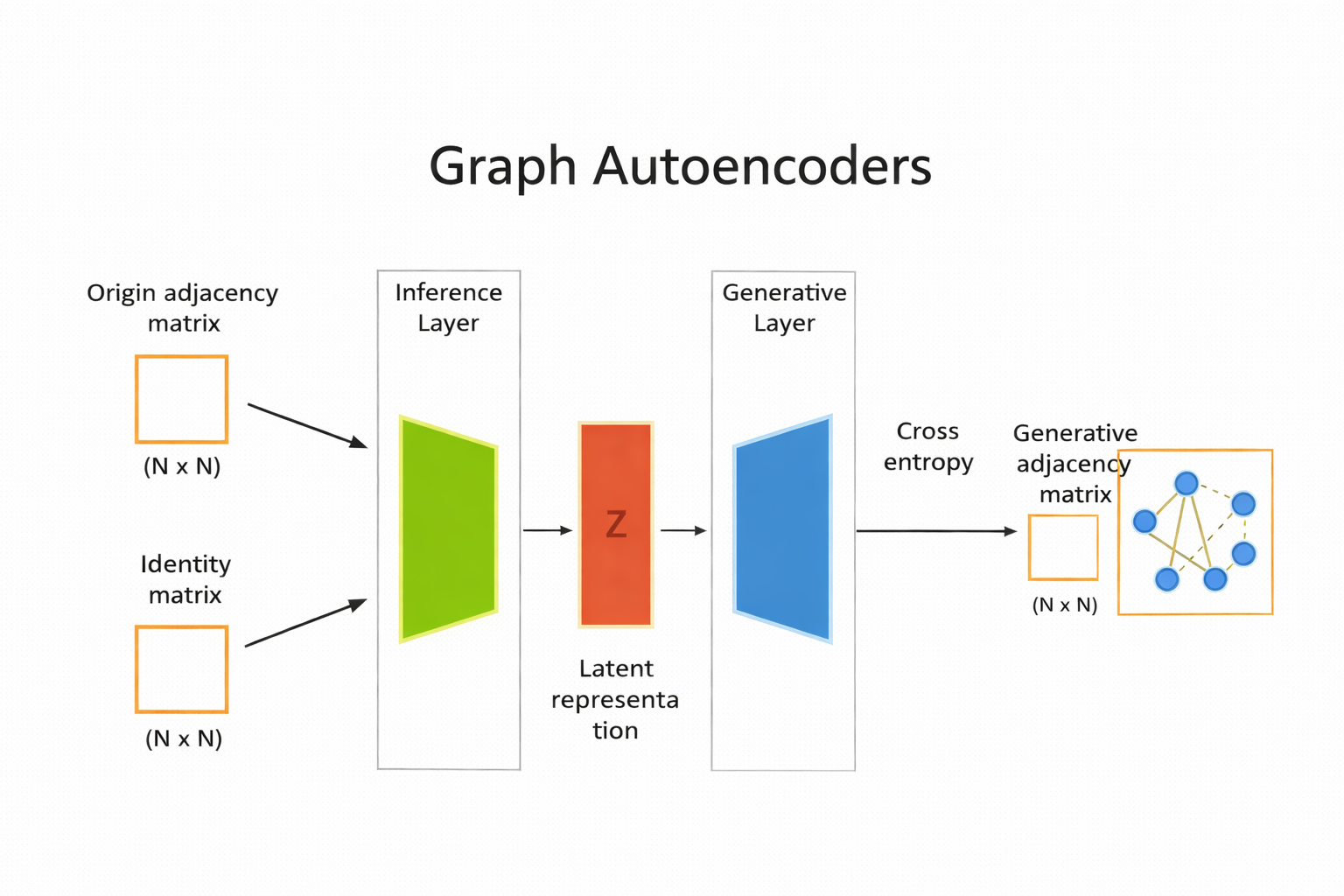
Graph Autoencoder#
specialized type of auto encoder designed to work with graph structured data. useful for tasks such as node clustering, link prediction, and graph generation.
from torch_geometric.datasets import Planetoid

citeseer_dataset = Planetoid(root = "Citeser_dataset", name = "Citeseer")

citeseer_dataset
# The Planetoid datasets (Cora/CiteSeer/PubMed) each contain a single graph
data = citeseer_dataset[0]

print(citeseer_dataset)
print(data)

# Optional: print key shapes
print("x (node features):", data.x.shape)          # [num_nodes, num_node_features]
print("edge_index (edges):", data.edge_index.shape) # [2, num_edges]
print("y (labels):", data.y.shape)                  # [num_nodes]
print("train/val/test masks:", data.train_mask.shape, data.val_mask.shape, data.test_mask.shape)
Citeseer()
Data(x=[3327, 3703], edge_index=[2, 9104], y=[3327], train_mask=[3327], val_mask=[3327], test_mask=[3327])
x (node features): torch.Size([3327, 3703])
edge_index (edges): torch.Size([2, 9104])
y (labels): torch.Size([3327])
train/val/test masks: torch.Size([3327]) torch.Size([3327]) torch.Size([3327])
CiteSeer is a classic citation network dataset used for node classification with GNNs.
Nodes = research papers
Edges = citation links between papers (paper A cites paper B)
Node features (data.x) = a bag-of-words style vector (each row represents one paper, each column represents a word/term feature).
Node labels (data.y) = the research topic/category of each paper (one label per node).
Masks (train_mask, val_mask, test_mask) = predefined splits that tell you which nodes to use for training, validation, and testing.
In PyTorch Geometric, Planetoid(…, name=”CiteSeer”) downloads and prepares the dataset, and citeseer_dataset[0] returns the single graph stored in the dataset.
Split data into train and test#
import torch
import torch_geometric.transforms as T
from torch_geometric.datasets import Planetoid

# Device (CPU or GPU)
device = torch.device("cuda" if torch.cuda.is_available() else "cpu")

# Define transformations
transform = T.Compose([
    T.NormalizeFeatures(),          # Normalize node feature vectors
    T.ToDevice(device),              # Move data to CPU/GPU
    T.RandomLinkSplit(
        num_val=0.10,                # 10% edges for validation
        num_test=0.20,               # 20% edges for testing
        neg_sampling_ratio=1.0,      # Equal number of negative edges
        is_undirected=True,          # Treat graph as undirected
        add_negative_train_samples=False
    )
])

# Load CiteSeer dataset with transform
citeseer_dataset = Planetoid(
    root="Citeseer_dataset",
    name="Citeseer",
    transform=transform
)

# After RandomLinkSplit, indexing returns (train, val, test)
train_data, val_data, test_data = citeseer_dataset[0]

# Print dataset splits
print("-" * 50)
print("Validation Data")
print(val_data)

print("-" * 50)
print("Test Data")
print(test_data)

print("-" * 50)
print("Train Data")
print(train_data)
Downloading https://github.com/kimiyoung/planetoid/raw/master/data/ind.citeseer.x
Downloading https://github.com/kimiyoung/planetoid/raw/master/data/ind.citeseer.tx
Downloading https://github.com/kimiyoung/planetoid/raw/master/data/ind.citeseer.allx
Downloading https://github.com/kimiyoung/planetoid/raw/master/data/ind.citeseer.y
Downloading https://github.com/kimiyoung/planetoid/raw/master/data/ind.citeseer.ty
Downloading https://github.com/kimiyoung/planetoid/raw/master/data/ind.citeseer.ally
Downloading https://github.com/kimiyoung/planetoid/raw/master/data/ind.citeseer.graph
Downloading https://github.com/kimiyoung/planetoid/raw/master/data/ind.citeseer.test.index
--------------------------------------------------
Validation Data
Data(x=[3327, 3703], edge_index=[2, 6374], y=[3327], train_mask=[3327], val_mask=[3327], test_mask=[3327], edge_label=[910], edge_label_index=[2, 910])
--------------------------------------------------
Test Data
Data(x=[3327, 3703], edge_index=[2, 7284], y=[3327], train_mask=[3327], val_mask=[3327], test_mask=[3327], edge_label=[1820], edge_label_index=[2, 1820])
--------------------------------------------------
Train Data
Data(x=[3327, 3703], edge_index=[2, 6374], y=[3327], train_mask=[3327], val_mask=[3327], test_mask=[3327], edge_label=[3187], edge_label_index=[2, 3187])
Processing...
Done!
import torch
from torch.nn import Module
from torch_geometric.nn import GCNConv

# -------------------------------
# Graph Autoencoder Model
# -------------------------------
class AutoEncoder(Module):
    def __init__(self, in_channels, hidden_channels, out_channels):
        super().__init__()

        # Encoder (GCN layers)
        self.conv1 = GCNConv(in_channels, hidden_channels)
        self.conv2 = GCNConv(hidden_channels, out_channels)

    def encode(self, x, edge_index):
        x = self.conv1(x, edge_index)
        x = x.relu()
        x = self.conv2(x, edge_index)
        return x  # latent node embeddings Z

    def decode(self, z, edge_label_index):
        # Inner product decoder
        return (z[edge_label_index[0]] * z[edge_label_index[1]]).sum(dim=-1)

    def decode_all(self, z):
        # Reconstruct full adjacency matrix
        prob_adj = z @ z.t()
        prob_adj = prob_adj.sigmoid()

        # Return only very confident edges
        return (prob_adj > 0.99).nonzero(as_tuple=False).t()


# -------------------------------
# Model setup
# -------------------------------
device = torch.device("cuda" if torch.cuda.is_available() else "cpu")

model = AutoEncoder(
    in_channels=citeseer_dataset.num_features,
    hidden_channels=128,
    out_channels=64
).to(device)

optimizer = torch.optim.Adam(model.parameters(), lr=0.01)
criterion = torch.nn.BCEWithLogitsLoss()

# -------------------------------
# Encode node embeddings
# -------------------------------
z = model.encode(train_data.x, train_data.edge_index)
print(z.shape)  # [num_nodes, latent_dim]
torch.Size([3327, 64])
z = model.encode(train_data.x , train_data.edge_index)
z.shape
torch.Size([3327, 64])
# ----------------------------------------
# 2) Instantiate model/optimizer/criterion
# ----------------------------------------
device = torch.device("cuda" if torch.cuda.is_available() else "cpu")

model = AutoEncoder(
    citeseer_dataset.num_features,
    hidden_channels=128,
    out_channels=64
).to(device)

optimizer = torch.optim.Adam(params=model.parameters(), lr=0.01)
criterion = torch.nn.BCEWithLogitsLoss()


# -----------------------------
# 3) Train step
# -----------------------------
from torch_geometric.utils import negative_sampling

def train():
    model.train()
    optimizer.zero_grad()

    z = model.encode(train_data.x, train_data.edge_index)

    # train_data.edge_label_index shape: (2, num_train_edges)
    # neg_edge_index shape: (2, num_train_edges)
    neg_edge_index = negative_sampling(
        edge_index=train_data.edge_index,
        num_nodes=train_data.num_nodes,
        num_neg_samples=train_data.edge_label_index.size(1)
    )

    # edge_label_index shape: (2, num_train_edges * 2)
    edge_label_index = torch.cat(
        [train_data.edge_label_index, neg_edge_index],
        dim=-1
    )

    # edge_label shape: (num_train_edges * 2)
    edge_label = torch.cat([
        train_data.edge_label,
        train_data.edge_label.new_zeros(neg_edge_index.size(1))
    ], dim=0)

    out = model.decode(z, edge_label_index).view(-1)
    loss = criterion(out, edge_label)
    loss.backward()
    optimizer.step()

    return loss


# -----------------------------
# 4) Test step (ROC-AUC)
# -----------------------------
from sklearn.metrics import roc_auc_score

@torch.no_grad()
def test(data):
    model.eval()

    z = model.encode(data.x, data.edge_index)
    out = model.decode(z, data.edge_label_index).view(-1).sigmoid()

    return roc_auc_score(
        data.edge_label.cpu().numpy(),
        out.cpu().numpy()
    )


# -----------------------------
# 5) Training loop
# -----------------------------
best_val_auc = final_test_auc = 0

for epoch in range(100):
    loss = train()

    val_auc = test(val_data)
    test_auc = test(test_data)

    if val_auc > best_val_auc:
        best_val_auc = val_auc
        final_test_auc = test_auc

    if (epoch + 1) % 10 == 0:
        print(
            f"Epoch: {epoch+1:03d}, Loss: {loss:.4f}, "
            f"Val AUC: {val_auc:.4f}, Test AUC: {test_auc:.4f}"
        )

print(f"Final Test AUC: {final_test_auc:.4f}")
Epoch: 010, Loss: 0.5807, Val AUC: 0.7597, Test AUC: 0.7830
Epoch: 020, Loss: 0.5213, Val AUC: 0.8127, Test AUC: 0.8321
Epoch: 030, Loss: 0.4988, Val AUC: 0.8564, Test AUC: 0.8685
Epoch: 040, Loss: 0.4753, Val AUC: 0.8449, Test AUC: 0.8626
Epoch: 050, Loss: 0.4546, Val AUC: 0.8560, Test AUC: 0.8842
Epoch: 060, Loss: 0.4503, Val AUC: 0.8544, Test AUC: 0.8868
Epoch: 070, Loss: 0.4416, Val AUC: 0.8642, Test AUC: 0.8968
Epoch: 080, Loss: 0.4393, Val AUC: 0.8665, Test AUC: 0.9009
Epoch: 090, Loss: 0.4368, Val AUC: 0.8595, Test AUC: 0.8947
Epoch: 100, Loss: 0.4365, Val AUC: 0.8604, Test AUC: 0.8935
Final Test AUC: 0.9008
z = model.encode(test_data.x, test_data.edge_index)
z
tensor([[-0.3211, -0.0390, -0.3111,  ...,  0.0044,  0.1391,  0.0499],
        [ 0.0751,  0.0498,  0.2231,  ..., -0.2271, -0.1097,  0.0576],
        [-0.2011, -0.1242, -0.1278,  ...,  0.1155,  0.0714, -0.0581],
        ...,
        [-0.4045, -0.0919, -0.0364,  ..., -0.1427,  0.0813,  0.1555],
        [-0.1620,  0.1902,  0.0524,  ..., -0.0284, -0.1536,  0.0007],
        [-0.1588, -0.0428,  0.1831,  ...,  0.0700, -0.0832, -0.0629]],
       grad_fn=<AddBackward0>)
z.shape
torch.Size([3327, 64])
final_edge_index = model.decode_all(z)
final_edge_index.shape
torch.Size([2, 4542])
self_loops = final_edge_index[0] == final_edge_index[1]

filterd_edges = final_edge_index[:,self_loops]
filterd_edges.shape
torch.Size([2, 80])
test_data.edge_index.shape
torch.Size([2, 7284])
Example#
import torch
import torch.nn.functional as F
import torch.nn as nn


from torch_geometric.datasets import QM9
from torch_geometric.loader import DataLoader
from torch_geometric.nn import NNConv, global_add_pool

import numpy as np
dset = QM9('.')
len(dset)
130831
The QM9 dataset contains approximately 134,000 small organic molecules, represented as graphs where:
Nodes correspond to atoms
Edges correspond to chemical bonds
Each molecule includes:
Atom features (e.g., atomic number)
Bond information
Multiple target properties such as energy, dipole moment, and molecular orbitals
data = dset[0]
data
Data(x=[5, 11], edge_index=[2, 8], edge_attr=[8, 4], y=[1, 19], pos=[5, 3], idx=[1], name='gdb_1', z=[5])
data.z
tensor([6, 1, 1, 1, 1])
data.new_attribute = torch.tensor([1, 2, 3])
data
Data(x=[5, 11], edge_index=[2, 8], edge_attr=[8, 4], y=[1, 19], pos=[5, 3], idx=[1], name='gdb_1', z=[5], new_attribute=[3])
device = torch.device("cuda:0" if torch.cuda.is_available() else "cpu")
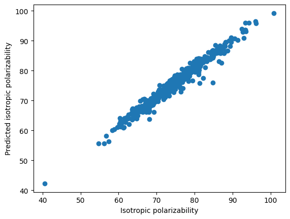
data.to(device)
data.new_attribute.is_cuda
False
class ExampleNet(torch.nn.Module):
    def __init__(self,num_node_features,num_edge_features):
        super().__init__()
        conv1_net = nn.Sequential(nn.Linear(num_edge_features, 32),
                                  nn.ReLU(),
                                  nn.Linear(32, num_node_features*32))
        conv2_net = nn.Sequential(nn.Linear(num_edge_features,32),
                                  nn.ReLU(),
                                  nn.Linear(32, 32*16))
        self.conv1 = NNConv(num_node_features, 32, conv1_net)
        self.conv2 = NNConv(32, 16, conv2_net)
        self.fc_1 = nn.Linear(16, 32)
        self.out = nn.Linear(32, 1)

    def forward(self, data):
        batch, x, edge_index, edge_attr=data.batch, data.x, data.edge_index, data.edge_attr
        x = F.relu(self.conv1(x, edge_index, edge_attr))
        x = F.relu(self.conv2(x, edge_index, edge_attr))
        x = global_add_pool(x,batch)
        x = F.relu(self.fc_1(x))
        output = self.out(x)
        return output
from torch.utils.data import random_split


train_set, valid_set, test_set = random_split(dset,[110000, 10831, 10000])

trainloader = DataLoader(train_set, batch_size=32, shuffle=True)
validloader = DataLoader(valid_set, batch_size=32, shuffle=True)
testloader = DataLoader(test_set, batch_size=32, shuffle=True)
qm9_node_feats, qm9_edge_feats = 11, 4
epochs = 4
net = ExampleNet(qm9_node_feats, qm9_edge_feats)

optimizer = torch.optim.Adam(net.parameters(), lr=0.01)
epochs = 4
target_idx = 1 # index position of the polarizability label
device = torch.device("cuda:0" if torch.cuda.is_available() else "cpu")
net.to(device)
ExampleNet(
  (conv1): NNConv(11, 32, aggr=add, nn=Sequential(
    (0): Linear(in_features=4, out_features=32, bias=True)
    (1): ReLU()
    (2): Linear(in_features=32, out_features=352, bias=True)
  ))
  (conv2): NNConv(32, 16, aggr=add, nn=Sequential(
    (0): Linear(in_features=4, out_features=32, bias=True)
    (1): ReLU()
    (2): Linear(in_features=32, out_features=512, bias=True)
  ))
  (fc_1): Linear(in_features=16, out_features=32, bias=True)
  (out): Linear(in_features=32, out_features=1, bias=True)
)
for total_epochs in range(epochs):

    epoch_loss = 0
    total_graphs = 0
    net.train()
    for batch in trainloader:
        batch.to(device)
        optimizer.zero_grad()
        output = net(batch)
        loss = F.mse_loss(output, batch.y[:, target_idx].unsqueeze(1))
        loss.backward()
        epoch_loss += loss.item()
        total_graphs += batch.num_graphs
        optimizer.step()

    train_avg_loss = epoch_loss / total_graphs
    val_loss = 0
    total_graphs = 0
    net.eval()
    for batch in validloader:
        batch.to(device)
        output = net(batch)
        loss = F.mse_loss(output,batch.y[:, target_idx].unsqueeze(1))
        val_loss += loss.item()
        total_graphs += batch.num_graphs
    val_avg_loss = val_loss / total_graphs


    print(f"Epochs: {total_epochs} | epoch avg. loss: {train_avg_loss:.2f} | validation avg. loss: {val_avg_loss:.2f}")
Epochs: 0 | epoch avg. loss: 0.55 | validation avg. loss: 0.21
Epochs: 1 | epoch avg. loss: 0.13 | validation avg. loss: 0.11
Epochs: 2 | epoch avg. loss: 0.11 | validation avg. loss: 0.18
Epochs: 3 | epoch avg. loss: 0.10 | validation avg. loss: 0.10
net.eval()
predictions = []
real = []

for batch in testloader:

    output = net(batch.to(device))
    predictions.append(output.detach().cpu().numpy())
    real.append(batch.y[:, target_idx].detach().cpu().numpy())

predictions = np.concatenate(predictions)
real = np.concatenate(real)
import matplotlib.pyplot as plt


plt.scatter(real[:500],predictions[:500])
plt.ylabel('Predicted isotropic polarizability')
plt.xlabel('Isotropic polarizability')
#plt.savefig('figures/18_12.png', dpi=300)
Text(0.5, 0, 'Isotropic polarizability')