Multilayer Perceptron (MLP) From Scratch#
In this section, we discuss the fundamental components of a feedforward neural network. Each component is derived mathematically and implemented explicitly using NumPy. No automatic differentiation or high-level abstractions are used; all gradients are computed manually to make the learning dynamics fully transparent.
We begin by defining a common interface for network layers, then implement linear transformations and nonlinear activation functions. Together, these components form the basis of forward propagation and backpropagation.
Mathematical Equations, Computational Graphs, and Backpropagation#
This notebook builds an MLP by defining Layer objects (Dense, ReLU, etc.) and composing them.
A layer maps:
\(\mathbf{y} = f(\mathbf{x}; \theta)\)
The MLP is a composition:
\(f(\mathbf{x}) = f_L \circ f_{L-1} \circ \dots \circ f_1(\mathbf{x})\)
Backpropagation is reverse-mode differentiation on the computational graph.
Dense (Fully Connected) Layer#
If we use mini-batches.
Batch size: (\(N\))
Input dimension: (\(d_{in}\))
Hidden dimension: (\(d_h\))
Output classes: (\(C\))
Forward#
For a batch input \(\mathbf{x} \in \mathbb{R}^{N \times d_{in}}\):
where:
\(\mathbf{W} \in \mathbb{R}^{d_{in} \times d_{out}}\)
\(\mathbf{b} \in \mathbb{R}^{d_{out}}\)
\(\mathbf{y} \in \mathbb{R}^{N \times d_{out}}\)
Computational graph (Dense)#
                            x ──┐
                                |
                            ├── MatMul ── z ── Add ── y
                                |               ▲
                            W ──┘               │
                                                b
Mathematically:
Backward (gradients)#
Assume upstream gradient:
Then:
Forward vs. Backward: values vs. sensitivities#
A feedforward neural network defines a composition of functions:
\(X \xrightarrow{f_1} H_1 \xrightarrow{f_2} H_2 \xrightarrow{} \cdots \xrightarrow{f_L} Z \xrightarrow{\text{loss}} L\)
Forward pass computes values of intermediate variables \(H_1, H_2, \dots, Z\) starting from the input \(X\).
Backward pass computes sensitivities (gradients) of the final scalar loss \(L\) with respect to intermediate variables and parameters.
Because \(L\) is a scalar, gradients like \(\partial L/\partial v\) have a direct interpretation:
\(\frac{\partial L}{\partial v} \quad\text{measures how a small change in } v \text{ would change the loss.}\)
This is why backpropagation naturally starts at the loss: the loss is the endpoint of the computational graph, and all parameters influence the loss only through the output.
Computational graph and the chain rule#
Backpropagation is the chain rule applied systematically.
If a variable \(u\) influences \(v\), and \(v\) influences the loss \(L\), then:
The operational principle is modular:
Each layer/module computes a forward mapping \(v = f(u;\theta)\).
During backward, if we know the upstream gradient \(G_{out}=\partial L/\partial v\), the layer can compute:
input gradient \(G_{in}=\partial L/\partial u\)
parameter gradients \(\partial L/\partial \theta\) (if the layer has parameters)
This is why you can say:
Given the gradient of the next layer, we can compute the gradient of the current layer.
It is simply the chain rule written in a reusable layer-by-layer form.
3. MLP notation (batch form)#
For a batch size \(N\):
\(H_0 = X \in \mathbb{R}^{N\times d_0}\)
For \(\ell=1,\dots,L\):
Affine (Dense) transform:
\[Z_\ell = H_{\ell-1} W_\ell + b_\ell \quad (W_\ell \in \mathbb{R}^{d_{\ell-1}\times d_\ell},\; b_\ell\in\mathbb{R}^{d_\ell}) \]Nonlinearity: $\( H_\ell = \phi(Z_\ell) \)$
Final logits are \(Z_L\). The training objective is a scalar loss \(L\) computed from \(Z_L\) and labels.
We want gradients for all parameters:
4. Why backward starts from the loss#
The loss \(L\) is a scalar function of the final model output. Every parameter affects \(L\) only through the sequence of intermediate computations.
Therefore the derivative propagation must begin at the endpoint:
Compute \(\partial L/\partial Z_L\) (loss gradient w.r.t. logits).
Propagate gradients backward through each layer:
\[\frac{\partial L}{\partial H_{L-1}},\; \frac{\partial L}{\partial Z_{L-1}},\; \dots,\; \frac{\partial L}{\partial H_0}\]At each layer, compute parameter gradients \(\partial L/\partial W_\ell\) and \(\partial L/\partial b_\ell\).
This is exactly the chain rule for a composition of functions, applied from right to left.
5. The reusable layer pattern#
Each layer exposes a backward mapping:
Input: upstream gradient \(G_{out}=\partial L/\partial (\text{layer output})\)
Outputs:
downstream gradient \(G_{in}=\partial L/\partial (\text{layer input})\)
parameter gradients \(\partial L/\partial \theta\) (if parameters exist)
In code, this corresponds to receiving grad_out and returning grad_in, while storing dW, db, etc.
6. Loss layer: Softmax + Cross-Entropy#
Let logits be \(Z\in\mathbb{R}^{N\times C}\), labels be one-hot \(Y\in\mathbb{R}^{N\times C}\).
Softmax:
Mean cross-entropy loss:
A key result (from differentiating softmax and cross-entropy together) is:
This gradient is the starting point of backpropagation into the network.
7. Activation layer: ReLU#
Forward:
Elementwise derivative:
Given upstream gradient \(G_H = \partial L/\partial H\), chain rule yields:
This shows why we cache \(Z\) in forward: the mask \(\mathbf{1}_{Z>0}\) is computed from it.
8. Dense (Affine) layer#
Forward: $\(Z = HW + b\)$
with \(H\in\mathbb{R}^{N\times d_{in}}\), \(W\in\mathbb{R}^{d_{in}\times d_{out}}\), \(b\in\mathbb{R}^{d_{out}}\), \(Z\in\mathbb{R}^{N\times d_{out}}\).
Let upstream gradient be \(G_Z = \partial L/\partial Z\). Then:
Weights $\(\boxed{\frac{\partial L}{\partial W} = H^\top G_Z}\)$
Bias
Inputs (to propagate further backward)
These are the core backprop equations used repeatedly throughout an MLP.
9. End-to-end example: two-layer MLP#
Consider:
Backward proceeds in reverse:
Loss → logits
Dense2 $\( \frac{\partial L}{\partial W_2}=H_1^\top G_{Z_2},\quad \frac{\partial L}{\partial b_2}=\sum_n (G_{Z_2})_{n,:},\quad G_{H_1}=G_{Z_2}W_2^\top \)$
ReLU1 $\( G_{Z_1}=G_{H_1}\odot \mathbf{1}_{Z_1>0} \)$
Dense1 $\( \frac{\partial L}{\partial W_1}=H_0^\top G_{Z_1},\quad \frac{\partial L}{\partial b_1}=\sum_n (G_{Z_1})_{n,:},\quad G_{H_0}=G_{Z_1}W_1^\top \)$
At the end, we have gradients for every parameter and can apply an optimizer update.
10. Why we cache forward values#
Backprop rules require certain forward intermediates:
Dense needs \(H\) to compute \(H^\top G_Z\)
ReLU needs \(Z\) to compute the mask \(\mathbf{1}_{Z>0}\)
Softmax+CE needs \(P\) (or logits \(Z\)) and labels
Therefore implementations store (cache) inputs/outputs during forward so that local derivatives can be computed efficiently during backward.
We define the following Basic class and utilize it in all layers.
import numpy as np

class Layer:
    def forward(self, x, training=True):
        raise NotImplementedError

    def backward(self, grad_out):
        raise NotImplementedError

    def params(self):
        return []

    def grads(self):
        return []

    def zero_grads(self):
        pass
class Dense(Layer):
    def __init__(self, in_features, out_features, weight_scale=0.01):
        self.W = weight_scale * np.random.randn(in_features, out_features)
        self.b = np.zeros(out_features)
        self.x = None  # cache
        self.dW = np.zeros_like(self.W)
        self.db = np.zeros_like(self.b)

    def forward(self, x, training=True):
        self.x = x
        return x @ self.W + self.b

    def backward(self, grad_out):
        # grad_out = dL/dy
        self.dW = self.x.T @ grad_out           # dL/dW
        self.db = grad_out.sum(axis=0)          # dL/db
        grad_x = grad_out @ self.W.T            # dL/dx
        return grad_x

    def params(self):
        return [self.W, self.b]

    def grads(self):
        return [self.dW, self.db]

    def zero_grads(self):
        self.dW.fill(0.0)
        self.db.fill(0.0)
3. ReLU(Rectified Linear Unit) Activation#
Forward#
The ReLU function outputs 0 if the input is less than zero, otherwise it will return the input itself: $\(f(x) = \text{ReLU}(x) = \max(0,x) \)$
ReLU helps introduce non-linearity into the model, which is essential for learning complex patterns.
It also helps avoid the vanishing gradient problem common in deep networks with the Sigmoid activation.
During backpropagation, only the gradients for inputs greater than 0 pass through:
Computational graph (Dense)#
x ── ReLU ── y
Backward#
The derivative is:
So:
class ReLU(Layer):
    def __init__(self):
        self.mask = None

    def forward(self, x, training=True):
        self.mask = (x > 0)
        return np.maximum(0, x)

    def backward(self, grad_out):
        return grad_out * self.mask
4. Building an MLP by Composing Layers (Sequential)#
If we build:
Then the computational graph is:
class Sequential(Layer):
    def __init__(self, *layers):
        self.layers = list(layers)

    def forward(self, x, training=True):
        for layer in self.layers:
            x = layer.forward(x, training=training)
        return x

    def backward(self, grad_out):
        for layer in reversed(self.layers):
            grad_out = layer.backward(grad_out)
        return grad_out

    def params(self):
        ps = []
        for layer in self.layers:
            ps.extend(layer.params())
        return ps

    def grads(self):
        gs = []
        for layer in self.layers:
            gs.extend(layer.grads())
        return gs

    def zero_grads(self):
        for layer in self.layers:
            layer.zero_grads()
5. Softmax + Cross-Entropy Loss#
Softmax (probabilities)#
Given logits \(\mathbf{z} \in \mathbb{R}^{N \times C}\): $\(p_{n,i} = \frac{e^{z_{n,i}}}{\sum_{j=1}^{C} e^{z_{n,j}}}\)$
Cross-entropy (integer class labels)#
If the true class for sample \(n\) is \(y_n\):
def softmax_cross_entropy_with_logits(logits, y):
    """
    logits: (N, C)
    y: (N,) integer labels
    returns: (loss, dlogits)
    """
    N, C = logits.shape

    # stable softmax
    z = logits - logits.max(axis=1, keepdims=True)
    exp_z = np.exp(z)
    probs = exp_z / exp_z.sum(axis=1, keepdims=True)

    # loss
    loss = -np.log(probs[np.arange(N), y] + 1e-12).mean()

    # gradient: (p - y_onehot)/N
    dlogits = probs.copy()
    dlogits[np.arange(N), y] -= 1.0
    dlogits /= N

    return loss, dlogits


def accuracy_from_logits(logits, y):
    pred = np.argmax(logits, axis=1)
    return (pred == y).mean()
6. Parameter Update (SGD)#
Gradient descent update:
We apply this to each parameter tensor in the model.
class SGD:
    def __init__(self, lr=1e-2, weight_decay=0.0):
        self.lr = lr
        self.weight_decay = weight_decay

    def step(self, model):
        params = model.params()
        grads = model.grads()

        for p, g in zip(params, grads):
            if self.weight_decay != 0.0:
                g = g + self.weight_decay * p
            p -= self.lr * g
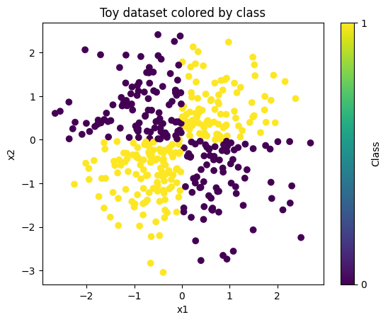
7. Toy Dataset (for demonstration)#
We’ll generate a simple 2D classification dataset.
This is not about dataset quality—just to verify:
forward works
backward gradients propagate
loss decreases during training
set_seed(0)

N = 400
X = np.random.randn(N, 2)

# non-linear target (quadrant-based)
y = (X[:, 0] * X[:, 1] > 0).astype(int)  # 0 or 1
---------------------------------------------------------------------------
NameError                                 Traceback (most recent call last)
Cell In[7], line 1
----> 1 set_seed(0)
      3 N = 400
      4 X = np.random.randn(N, 2)

NameError: name 'set_seed' is not defined
import matplotlib.pyplot as plt

# Assumes you already have:
# X: shape (N, 2)
# y: shape (N,) with values 0 or 1

X_plot = np.asarray(X)
y_plot = np.asarray(y).reshape(-1)

plt.figure()
sc = plt.scatter(X_plot[:, 0], X_plot[:, 1], c=y_plot)  # colors by class label
plt.xlabel("x1")
plt.ylabel("x2")
plt.title("Toy dataset colored by class")
plt.colorbar(sc, ticks=[0, 1], label="Class")
plt.show()
8. Build and Train the MLP#
Model:
Training loop:
Forward: logits
Loss + gradient: \(L, \frac{\partial L}{\partial \mathbf{z}}\)
Backward through model
SGD update
set_seed(0)

model = Sequential(
    Dense(2, 64, weight_scale=0.1),
    ReLU(),
    Dense(64, 64, weight_scale=0.1),
    ReLU(),
    Dense(64, 2, weight_scale=0.1),
)

opt = SGD(lr=1e-2, weight_decay=1e-4)

for epoch in range(1, 301):
    # forward
    logits = model.forward(X, training=True)

    # loss + initial gradient
    loss, dlogits = softmax_cross_entropy_with_logits(logits, y)

    # backward
    model.zero_grads()
    model.backward(dlogits)

    # update
    opt.step(model)

    if epoch % 50 == 0:
        acc = accuracy_from_logits(model.forward(X, training=False), y)
        print(f"epoch={epoch:3d}  loss={loss:.4f}  acc={acc:.3f}")
epoch= 50  loss=0.6870  acc=0.655
epoch=100  loss=0.6803  acc=0.685
epoch=150  loss=0.6734  acc=0.685
epoch=200  loss=0.6651  acc=0.698
epoch=250  loss=0.6565  acc=0.710
epoch=300  loss=0.6478  acc=0.720
set_seed(0)

batch_size = 64
epochs = 300
N = X.shape[0]

for epoch in range(1, epochs + 1):
    # shuffle indices each epoch
    idx = np.random.permutation(N)
    X_shuf = X[idx]
    y_shuf = y[idx]

    epoch_loss = 0.0
    epoch_acc = 0.0
    num_batches = 0

    for start in range(0, N, batch_size):
        end = start + batch_size
        Xb = X_shuf[start:end]
        yb = y_shuf[start:end]

        # forward
        logits = model.forward(Xb, training=True)

        # loss + initial gradient (scaled by batch size internally)
        loss, dlogits = softmax_cross_entropy_with_logits(logits, yb)

        # backward + update
        model.zero_grads()
        model.backward(dlogits)
        opt.step(model)

        # bookkeeping
        epoch_loss += loss
        epoch_acc += accuracy_from_logits(logits, yb)
        num_batches += 1

    if epoch % 50 == 0:
        print(f"epoch={epoch:3d}  loss={epoch_loss/num_batches:.4f}  acc={epoch_acc/num_batches:.3f}")
epoch= 50  loss=0.5670  acc=0.770
epoch=100  loss=0.4515  acc=0.868
epoch=150  loss=0.3135  acc=0.922
epoch=200  loss=0.2291  acc=0.949
epoch=250  loss=0.1729  acc=0.973
epoch=300  loss=0.1395  acc=0.984
9. Student Checklist (Understanding Backprop)#
Students should be able to explain:
Why Dense backward gives: $\(\frac{\partial L}{\partial \mathbf{W}} = \mathbf{x}^T \frac{\partial L}{\partial \mathbf{y}}\)$
Why ReLU backward uses a mask:
\[\frac{\partial L}{\partial x} = \frac{\partial L}{\partial y}\odot \mathbb{1}_{x>0}\]Why softmax + cross-entropy gradient simplifies to:
\[\frac{\partial L}{\partial \mathbf{z}} = \frac{1}{N}(\mathbf{p}-\mathbf{Y})\]How the computational graph explains the chain rule:
\[\frac{\partial L}{\partial u} = \sum_{v} \frac{\partial L}{\partial v}\frac{\partial v}{\partial u}\]
Backpropagation and Gradient Flow in a Multilayer Perceptron#
This section provides a consolidated view of how gradients flow through the network, from the loss function back to each layer’s parameters.
Gradient Flow Diagram (Forward and Backward)#
Forward pass#
                                        X (input batch)
                                           │
                                           ▼
                                        Dense1: Z1 = XW1 + b1
                                           │
                                           ▼
                                        ReLU1:  A1 = max(0, Z1)
                                           │
                                           ▼
                                        Dense2: Z2 = A1W2 + b2
                                           │
                                           ▼
                                        ReLU2:  A2 = max(0, Z2)
                                           │
                                           ▼
                                        Dense3: Z3 = A2W3 + b3   (logits)
                                           │
                                           ▼
                                        Softmax + Cross-Entropy Loss L
Backward pass (reverse order)#
                                        ∂L/∂Z3  (from loss)
                                           │
                                           ├── ∂L/∂W3 , ∂L/∂b3
                                           ▼
                                        ∂L/∂A2 = ∂L/∂Z3 · W3ᵀ
                                           │
                                           ▼
                                        ReLU mask (Z2 > 0)
                                           │
                                           ▼
                                        ∂L/∂Z2
                                           │
                                           ├── ∂L/∂W2 , ∂L/∂b2
                                           ▼
                                        ∂L/∂A1 = ∂L/∂Z2 · W2ᵀ
                                           │
                                           ▼
                                        ReLU mask (Z1 > 0)
                                           │
                                           ▼
                                        ∂L/∂Z1
                                           │
                                           ├── ∂L/∂W1 , ∂L/∂b1
                                           ▼
                                        ∂L/∂X
Consolidated Backpropagation Mathematics#
Consider a minibatch:
Input: \( X \in \mathbb{R}^{N \times d_{in}} \)
Labels: \( y \in \{0,\dots,C-1\}^N \)
The MLP is defined as:
\(\begin{aligned} Z_1 &= XW_1 + b_1 \\ A_1 &= \mathrm{ReLU}(Z_1) \\ Z_2 &= A_1W_2 + b_2 \\ A_2 &= \mathrm{ReLU}(Z_2) \\ Z_3 &= A_2W_3 + b_3 \end{aligned}\)
Step 1: Softmax + Cross-Entropy Gradient#
\(P = \mathrm{softmax}(Z_3)\)
\(L = -\frac{1}{N}\sum_{n=1}^N \log P_{n,y_n}\)
The gradient with respect to logits is:
\(\frac{\partial L}{\partial Z_3} = \frac{1}{N}(P - Y)\)
This gradient is the starting point of backpropagation.
Step 2: Dense Layer Backpropagation#
For a dense layer:
\(Z = AW + b\)
Given upstream gradient \(G = \frac{\partial L}{\partial Z} \):
\(\begin{aligned} \frac{\partial L}{\partial W} &= A^\top G \\ \frac{\partial L}{\partial b} &= \sum_{n=1}^N G_{n,:} \\ \frac{\partial L}{\partial A} &= G W^\top \end{aligned}\)
This applies to all Dense layers in the network.
Step 3: ReLU Backpropagation#
\(A = \mathrm{ReLU}(Z)\)
The derivative of ReLU is:
\(\frac{\partial A}{\partial Z} = \begin{cases} 1 & Z > 0 \\ 0 & Z \le 0 \end{cases}\)
Thus: \(\frac{\partial L}{\partial Z} = \frac{\partial L}{\partial A} \odot \mathbf{1}[Z > 0]\)
ReLU has no parameters, but it gates gradient flow.
End-to-End Backpropagation Summary#
The loss function provides \( \frac{\partial L}{\partial Z_3} \)
Each Dense layer computes gradients for its weights, bias, and inputs
Each ReLU layer applies a binary mask
Gradients propagate backward via the chain rule
The optimizer updates parameters using stored gradients
This mirrors exactly how the backward() methods are composed in the code.